
AIRFOILS 3D ROTATIONS IN LEPARAGLIDING
Study of geometric transformations to rotate airfoils in three axes
1.
Motivation
2. Airfoil rotations in space
3. A bit of analytical geometry in space
4. Graphic OpenSCAD experimentation and study of the movements and their compositions
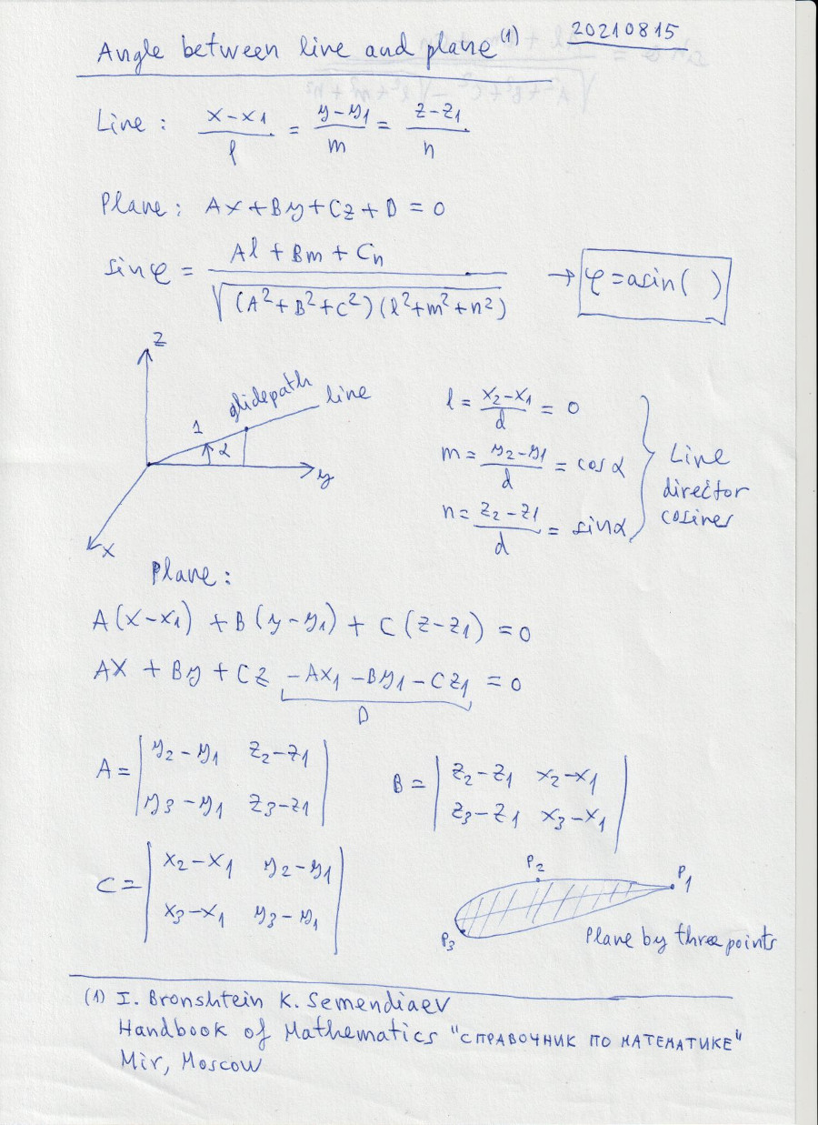
5. Angle phi between line and plane
6. Angle chi between two lines in space
7. Example
1. Motivation
Define geometrically a paraglider wing, basically is to locate airfoils in the space with the appropiate rotations, traslacions, and factors of the scale. Program LEparagliding until versions 3.15 rotates the airfoils in two axes:
- First rotation on an axis perpendicular to the profile plane (axis parallel to "X"), to achieve the desired relative angle of incidence "washin" assuming the wing is flat and the airfoils parallel to each other.
- Second rotation on an axis coinciding with the profile chord before the first rotation, (axis parallel to "Y")
This system is simple, works, and allows us to define excellent wings. However, some time ago I think in a third rotation, a rotation around the vertical axis "Z", which implies that the ribs are not all parallel to each other in the planform scheme.
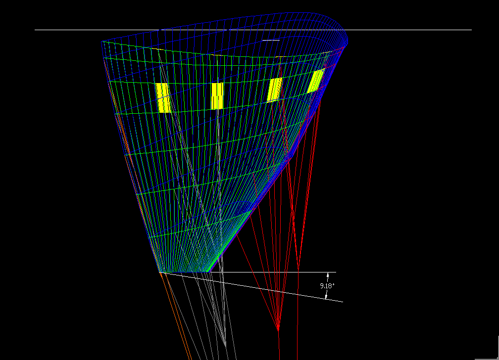
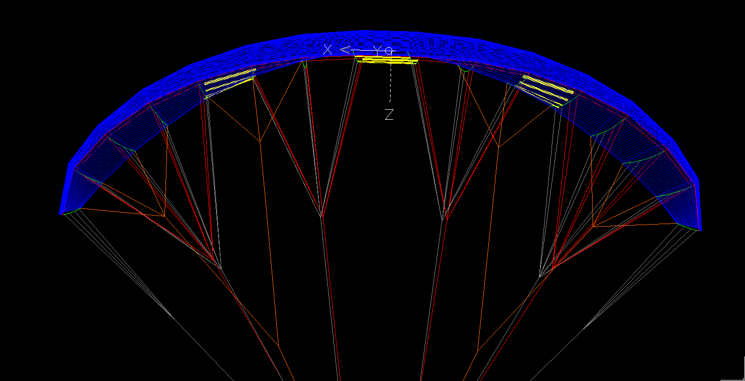
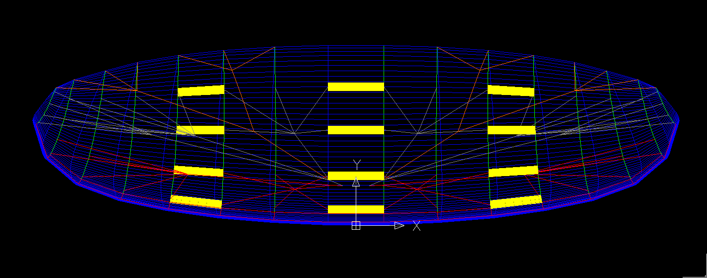
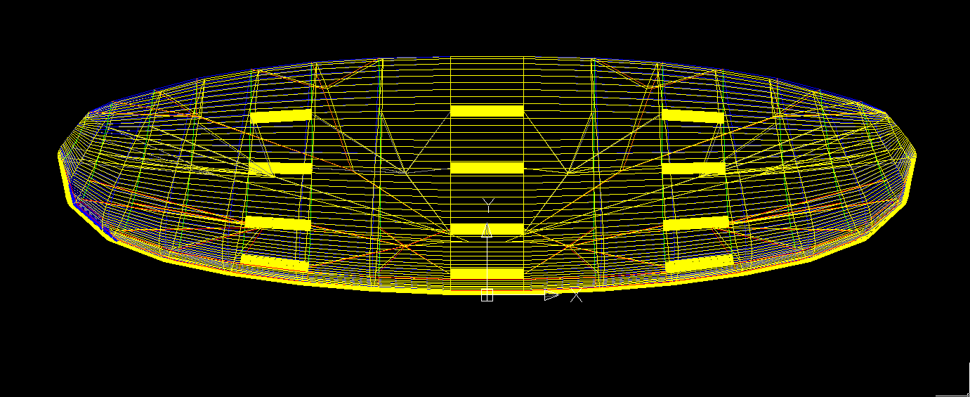
Talking with Arnaud Martinez about his new design, the Stork, made me realize that the additional rotation around "Z" axis can be useful to insert the airfoils within the glide trajectory. That is to say, to ensure that the line of trajectory is contained in the airfoil plane, so the flow will cross the airfoil according to the calculated shape. Of course, we can adjust the angles in the "Z" to obtain other effects.
So soon we will add two additional columns to define the geometry of the wing in SECTION 1, one for the angle Z, and the other to set the position of the axis of rotation with respect to the % chord...

Figure 1. This scheme is used to realize the importance of aligning the airfoils according to the glide path. The central airfoil (A) is in a vertical plane, and therefore the trajectory of the flight is contained within. The wingtip airfoil (C), may be in a completely horizontal plane. Thus, it is not well inserted into the glide path. If we do a rotation equal to the glide angle in an horizontal axis (vertical local axis of the airfoil), we get the glide path inside the airfoil plane. So the aerodynamic performance will be maximum. For a generic airfoil (B) it will be necessary to do an intermediate rotation.
2. Airfoil rotations in space
To add a third rotation in the space, I have to check the code currently used by the program, and especially to analyze in what order to apply the rotations and with what reference points do not create a mess. This is what I'm currently doing.
We consider the orthonormal axes x,y,z as the local airfoil axes content in the plane yz. The rotated airfoil will have the local axes x',y',z'. And the three rotations to consider are the following:


Figure 3. Definition of the director cosines, used in the matrix of rotation of coordinate systems.
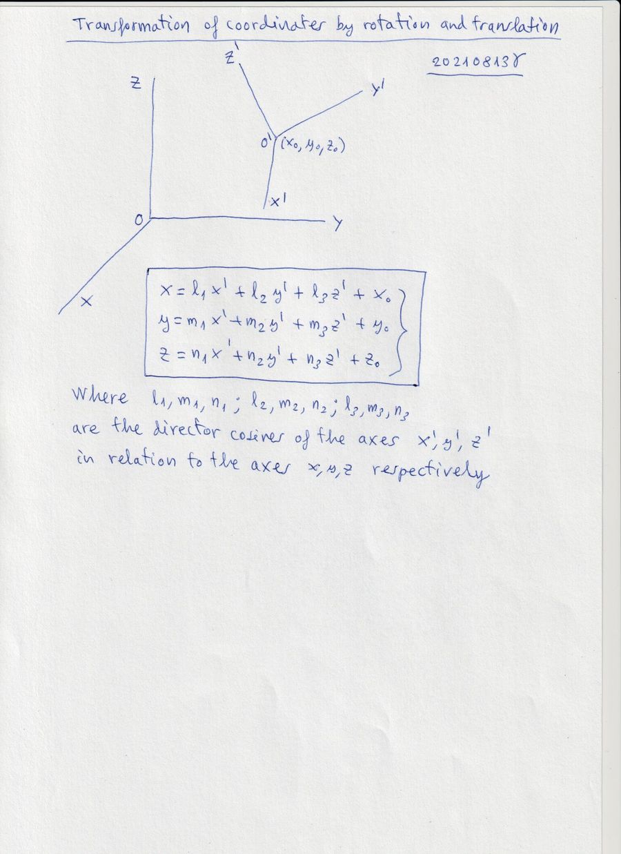
Figure 4. General transformation of coordinates in the space, by rotation and translation.
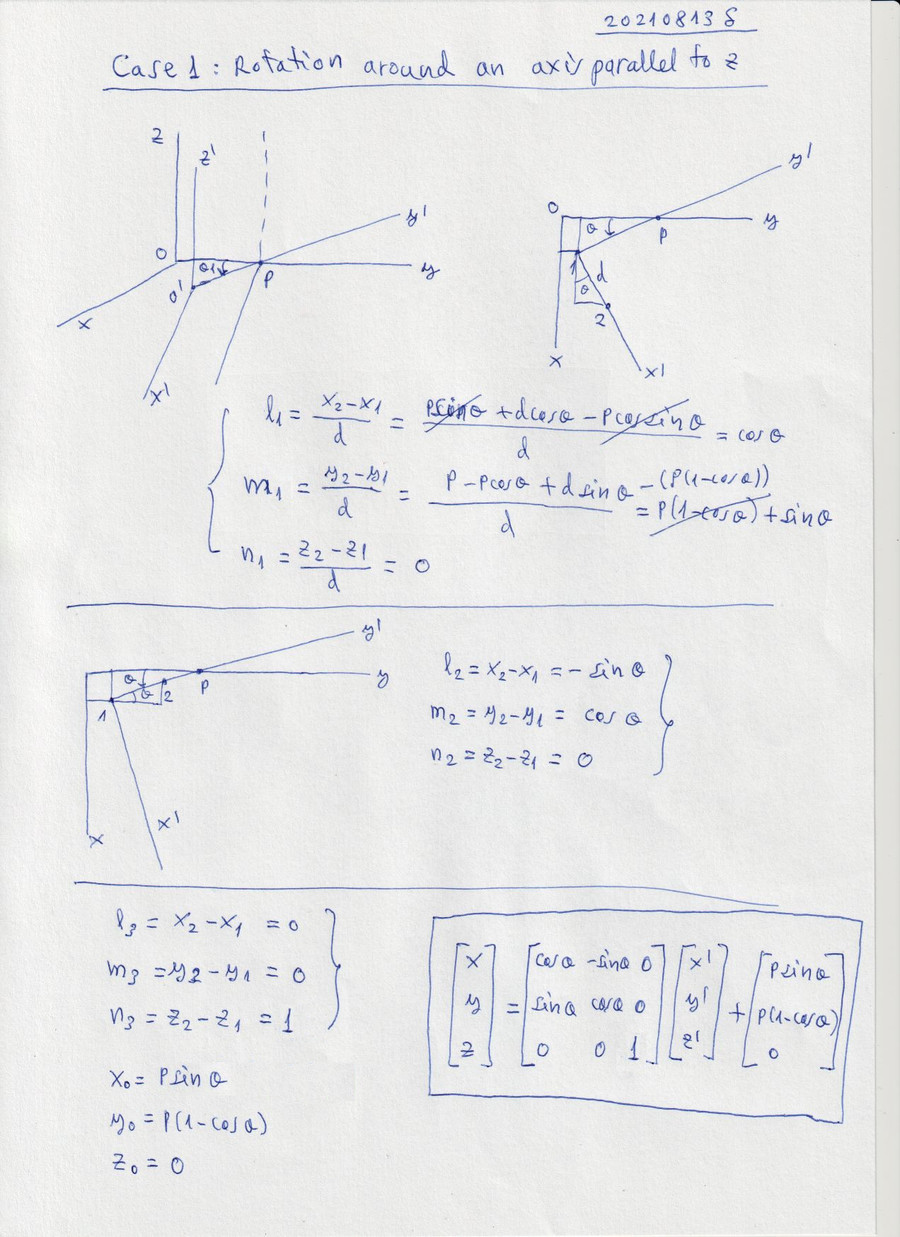
Figure 5. We obtain the coordinates transformation in the case of a rotation around an axis parallel to Z.

Figure 6. We obtain the coordinates transformation in the case of a rotation around an axis parallel to X.

Figure 7. We obtain the coordinates transformation in the case of a rotation around Y axis.
Well, now we have the analytic expressions for the coordinate transformation for any of the rotations. The next step is to define the order of application of the rotations and with respect to which axes. This is important to ensure compatibility with previous versions of LEparagliding and not to get strange results. When Z-rotations are defined as zero, the results of the 3D model must be exactly the same as in previous versions.
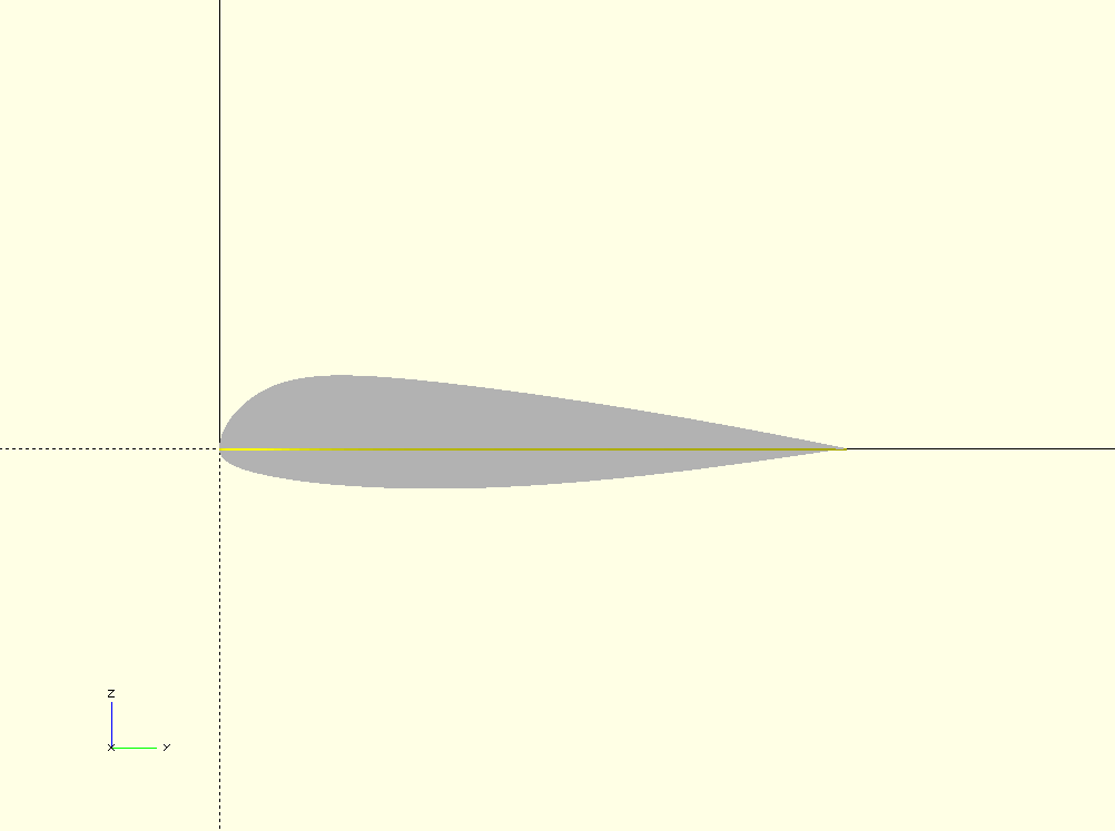
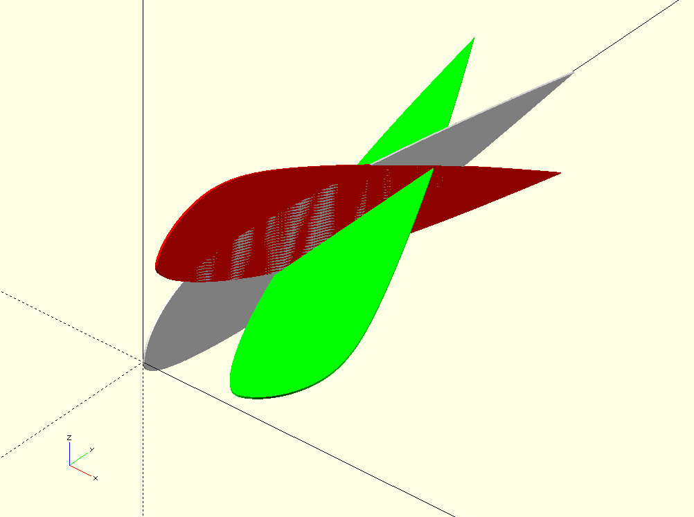
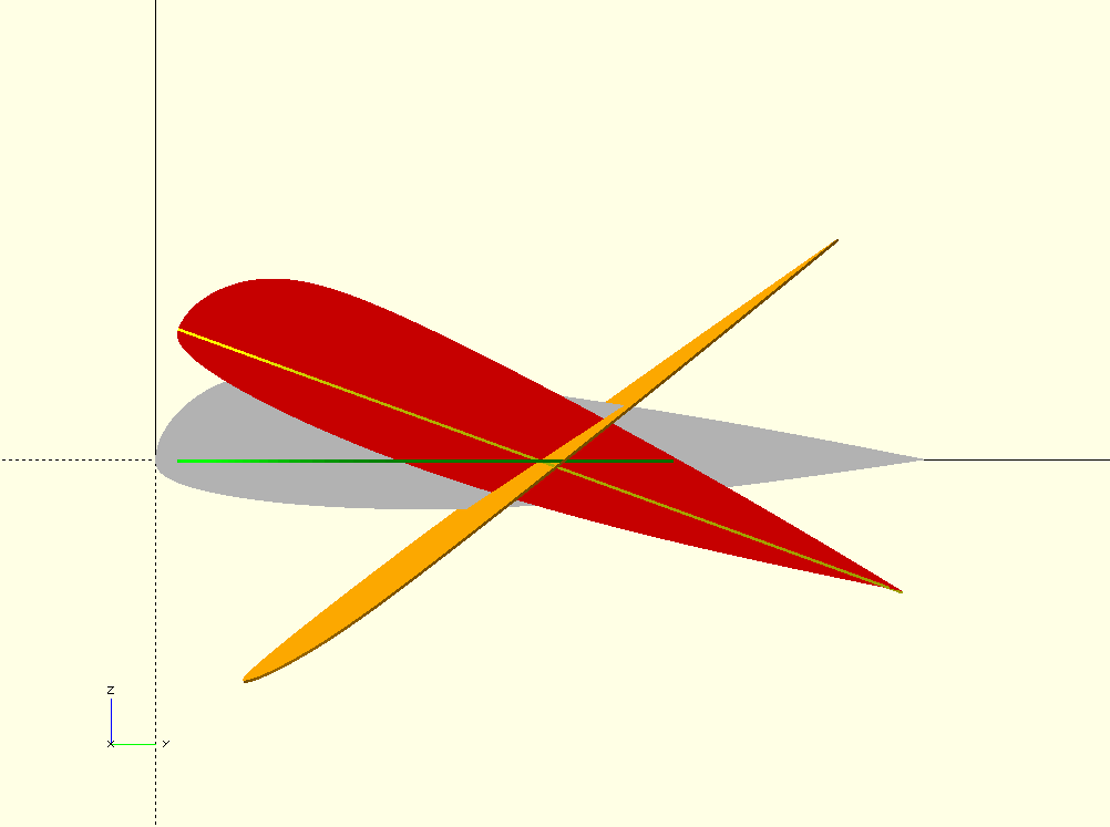
4. Graphic experimentation and study of the movements and their compositions, using openscad
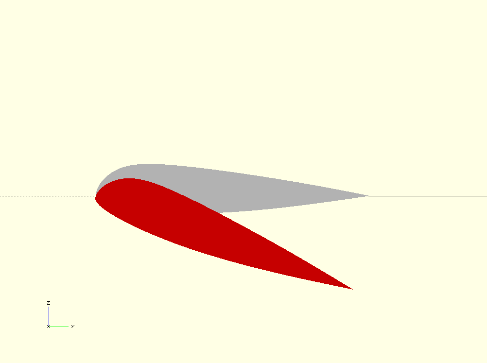
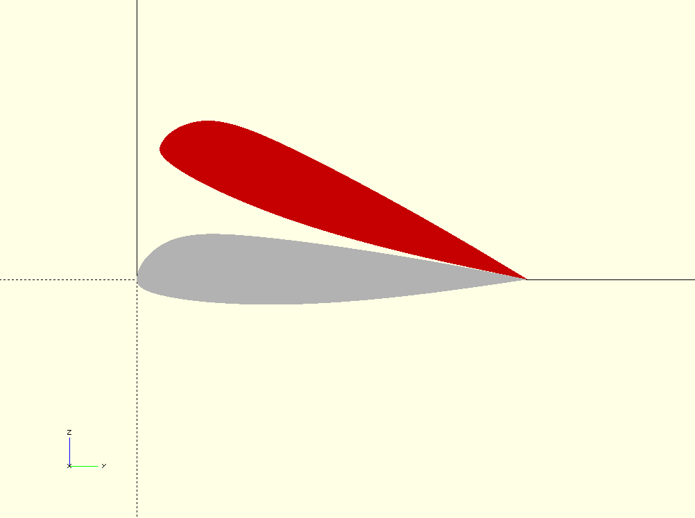
Before applying the rotation formulas, it is necessary to analyze in detail what is the effect of each of the rotations with respect to the axes considered and how influences the order of application. We modeled a gnuLAB3.dxf profile with the OpenSCAD program and visualized the movements. OpenSCAD is ideal for doing graphical experiments of this type. Here the OpenSCAD script and all files in .zip fomat here.
2. Airfoil rotations in space
3. A bit of analytical geometry in space
4. Graphic OpenSCAD experimentation and study of the movements and their compositions
5. Angle phi between line and plane
6. Angle chi between two lines in space
7. Example
1. Motivation
Define geometrically a paraglider wing, basically is to locate airfoils in the space with the appropiate rotations, traslacions, and factors of the scale. Program LEparagliding until versions 3.15 rotates the airfoils in two axes:
- First rotation on an axis perpendicular to the profile plane (axis parallel to "X"), to achieve the desired relative angle of incidence "washin" assuming the wing is flat and the airfoils parallel to each other.
- Second rotation on an axis coinciding with the profile chord before the first rotation, (axis parallel to "Y")
This system is simple, works, and allows us to define excellent wings. However, some time ago I think in a third rotation, a rotation around the vertical axis "Z", which implies that the ribs are not all parallel to each other in the planform scheme.
Talking with Arnaud Martinez about his new design, the Stork, made me realize that the additional rotation around "Z" axis can be useful to insert the airfoils within the glide trajectory. That is to say, to ensure that the line of trajectory is contained in the airfoil plane, so the flow will cross the airfoil according to the calculated shape. Of course, we can adjust the angles in the "Z" to obtain other effects.
So soon we will add two additional columns to define the geometry of the wing in SECTION 1, one for the angle Z, and the other to set the position of the axis of rotation with respect to the % chord...
Figure 1. This scheme is used to realize the importance of aligning the airfoils according to the glide path. The central airfoil (A) is in a vertical plane, and therefore the trajectory of the flight is contained within. The wingtip airfoil (C), may be in a completely horizontal plane. Thus, it is not well inserted into the glide path. If we do a rotation equal to the glide angle in an horizontal axis (vertical local axis of the airfoil), we get the glide path inside the airfoil plane. So the aerodynamic performance will be maximum. For a generic airfoil (B) it will be necessary to do an intermediate rotation.
2. Airfoil rotations in space
To add a third rotation in the space, I have to check the code currently used by the program, and especially to analyze in what order to apply the rotations and with what reference points do not create a mess. This is what I'm currently doing.
We consider the orthonormal axes x,y,z as the local airfoil axes content in the plane yz. The rotated airfoil will have the local axes x',y',z'. And the three rotations to consider are the following:
Figure 3. Definition of the director cosines, used in the matrix of rotation of coordinate systems.
Figure 4. General transformation of coordinates in the space, by rotation and translation.
Figure 5. We obtain the coordinates transformation in the case of a rotation around an axis parallel to Z.
Figure 6. We obtain the coordinates transformation in the case of a rotation around an axis parallel to X.
Figure 7. We obtain the coordinates transformation in the case of a rotation around Y axis.
Well, now we have the analytic expressions for the coordinate transformation for any of the rotations. The next step is to define the order of application of the rotations and with respect to which axes. This is important to ensure compatibility with previous versions of LEparagliding and not to get strange results. When Z-rotations are defined as zero, the results of the 3D model must be exactly the same as in previous versions.
4. Graphic experimentation and study of the movements and their compositions, using openscad
Before applying the rotation formulas, it is necessary to analyze in detail what is the effect of each of the rotations with respect to the axes considered and how influences the order of application. We modeled a gnuLAB3.dxf profile with the OpenSCAD program and visualized the movements. OpenSCAD is ideal for doing graphical experiments of this type. Here the OpenSCAD script and all files in .zip fomat here.


