LEPARAGLIDING 3.29 "Jardins"
USER MANUAL

1. INTRODUCTION

2. GENERAL CONCEPTS

3. FILES ASSOCIATED WITH THE PROGRAM

4. HOW TO WORK WITH THE PROGRAM

5. COMPOSITION OF THE AIRFOIL FILE

6. COMPOSITION OF THE INPUT DATA FILE leparagliding.txt

FIGURE INDEX

1. INTRODUCTION

This manual describes the use of LEparagliding created by Laboratori d'envol for the design of paragliders. The author of the program provides no other information as described in the web. There is no warranty for the correct operation of the program. You assume the full consequences of use of the program.

LEparagliding is very "cryptic" to use, "FORTRAN style", but very powerful. FORTRAN is a programming language aimed at numerical calculation, which means FORmula TRANslation. It is a language that allows us to accurately translate the ideas of geometry and mathematics to a code that produces amazing graphical and numerical results.

The program implements the theoretical developed in the book "Paraglider Design Handbook", which is advisable to study, because many of the contents are complementary.

I apologize, because this manual provides explanations in a style slightly rough. It is possible that some subjects are poorly explained. I will be happy to provide further clarification by pm. The program is not perfect, but it works.


2. GENERAL CONCEPTS

LEparagliding is a calculation engine written in GNU FORTRAN language, that performs the reading the data of the input files, and writes the results to the output files.

Input files:

Output files:


3. FILES ASSOCIATED WITH THE PROGRAM


4. HOW TO WORK WITH THE PROGRAM

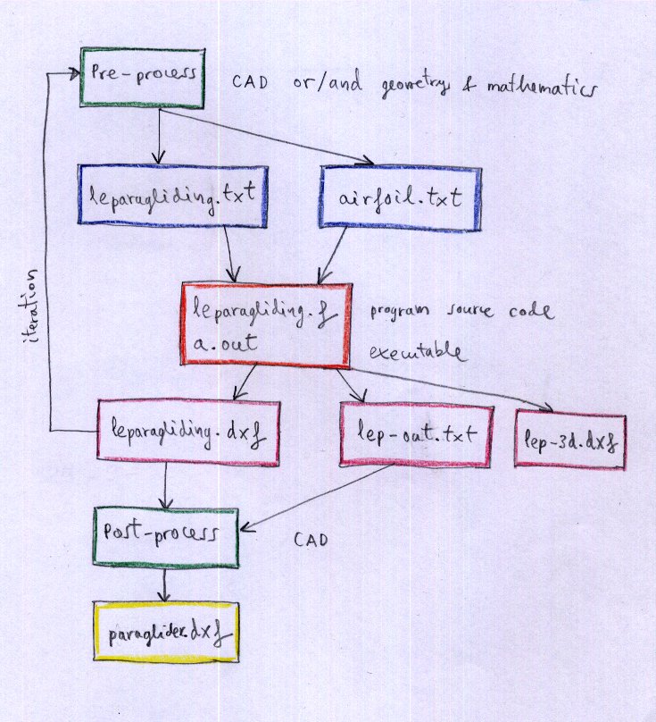
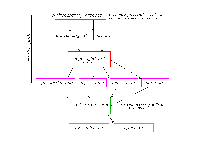
Working with LEparagliding consists of the following phases:

  1. Pre‑process – It is the initial phase of design, whether using CAD or pencil and graph paper and calculator. It defines the shape in plan, the lobe or vault and the desired inclination of the ribs. An analytical pre‑processor is available (is optional, and not strictly necessary), but very practical.
  2. Edit data file – Described below in detail. Complete sections 1 to 31. It is the most important operation, and the overall design of the glider itself.
  3. Program execution (seconds) – GNU/Linux: run ./lep-X.XX.out in a terminal. Windows: execute lep-X.XX.exe including one or more compatible cygwin .dll's in the same directory (or run ./lep-X.XX.out in a Cygwin terminal without the dll's). Mac OSX: compile source code in a terminal: "f77 leparagliding.f" and run "./lep-X.XX.out" in terminal as in linux (compiler name will be f77, g77, gfortran, or equivalent). Not tested yet.
  4. Viewing the drawings (CAD) – The program CAD displays the results dxf file. Please use 'zoom_extension' command.
  5. Iteration from stage 1 to achieve the desired layout.
  6. Post‑process CAD – Drawings can be edited by the CAD program to improve the presentation. They should position the panels and ribs on a reference template and print the templates in an array of A4/A3 size paper or plotter.

leparagliding workflow

Figure 1: How to work with the program.

Since 2.23 version and additional file lines.txt is in the output.
Since 2.28 version and additional file run-log.txt is in the output.
.tex file still not available.


5. COMPOSITION OF THE AIRFOIL FILES

The file of the profile data must have the following structure:

The coordinates are ordered starting at the trailing edge, covering the top surface, passed through the leading edge and coming through the lower surface and again ending at the trailing edge.

Important: The endpoint of the extrados must exactly match the start in % of the opening (air inlet), and the starting point of the intrados must exactly match the end in % of the opening (air outlet). Therefore the airfoil must be processed prior in a CAD program to achieve this. Therefore if you want to vary the start and end points of the air openings along span, you must detail specific profiles for this. Init and end points of openings declared in leparagliding.txt file must be consistent with the selected airfoils.

airfoil leparagliding

Figure 2: Airfoils definition

It is essential that the number of points of extrados, openings, and intrados, and all are exactly the same for all profiles defined in a wing model.
The maximum number of points allowed per profile is 500.

Zero‑thickness wingtip airfoil:

Usually, you must define a profile of zero thickness for the final profile of the wingtip. It is advisable to move the end of the panel's top surface (upper panel) to 0% of the profile, and keep the same number of points for each item (upper panel "extrados", air intakes, bottom panel "intrados"). This zero thickness profile is not necessary to define if we use the amplification coefficients of section 30 so that the coefficient applied to the last profile is 0.0.


6. COMPOSITION OF THE INPUT DATA FILE

Designing the paraglider is simplified to editing the file leparagliding.txt either creating it from scratch or, most commonly and recommended, by editing an existing model.

Very important, to take into account:

  • All lines that begin with the symbol "*" are comments that are not used by the program, although you must maintain it to keep the sequence of reading.
  • It is not allowed to add blank lines.
  • Each line must contain the expected number of parameters and from the expected type (integer, real, text, boolean).
  • Once the expected parameters have been completed, comments can be added to the same line, which will not be read by the program.

The main units planned for the data file are centimeters (cm), except sewing allowances in section 6, and some values in section 20 and 21 will be expressed in mm. Optionally, you could use inches and tenths of inches, but this has not been tested ever and not recommended.

You must fill in all the necessary parameters section by section until the end of the file, following this manual. I insist that the most practical thing is always to start with an existing template.

For each line of the data file, we will explain the type of parameter and its meaning. The graphic diagrams are very important to understand what type of parameter we are referring to. The order, data type, and number of rows is essential for a correct reading of the data file.

SECTION 1: GEOMETRY

Lines 1‑8:

* LABORATORI D'ENVOL PARAGLIDING DESIGN          *
* Input data file 3.28 version                   *
**************************************************************
* Version 2026-05-01                              *
**************************************************************
*                    1. GEOMETRY                  *
**************************************************************
      

Lines 9 to 24:

  • text : Brand name (between " ")
  • text : Wing name (between " ")
  • real : Drawing scale (1.0 usual value)
  • real : Wing scale (1.0 usual value)
  • integer : Cells number
  • integer : Ribs number
  • real1 integer real2 : Alpha wingtip, parameter, (alpha center) – see description below.
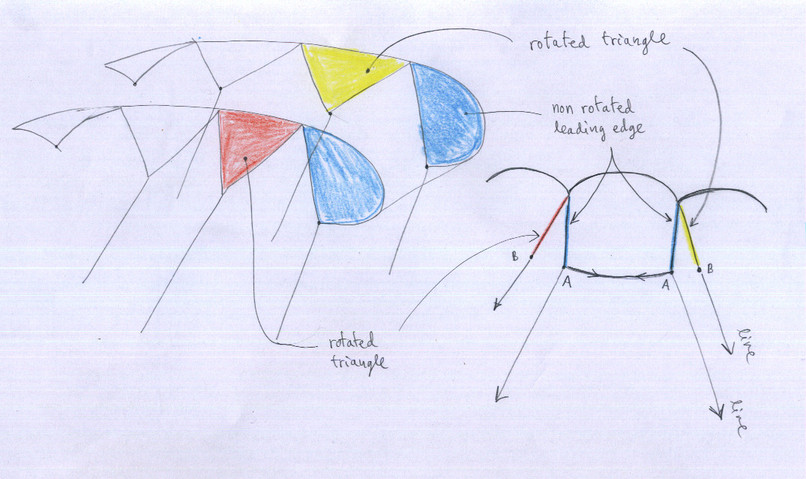
  • text boolean : Paraglider type "ds" double surface, "ss" single surface, or "pc" parachute. Boolean set to 0 or 1. If 1 then leading edge triangles will be not rotated (only used in ss paragliders).

Alpha wingtip, parameter, (alpha center):

real1: Maximum torsion angle (washin) between central airfoil and tips.
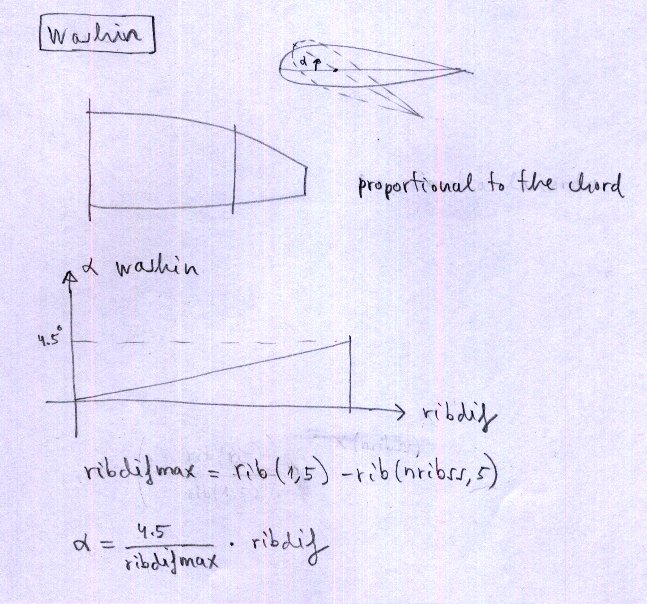
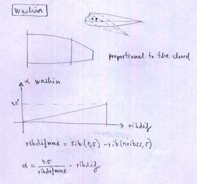
integer: 0, 1, or 2. If 0 → manual washin; if 1 → washin proportional to chord, maximum at tip; if 2 → automatic washin from center to tip (first real is tip washin, last real is center washin).
real2: angle of attack in the center (only for case 2).

Example: 3.5   2  -1.0 → tip AoA 3.5°, case 2, center AoA -1.0°. Distribution proportional to chord.

Paraglider type:

"ds": double surface airfoils (intrados and extrados)
"ss": single skin paragliders – intrados not drawn, but need special sawtooth profile.
"pc": parachutes using double surface airfoils.

boolean: set to 0 or 1. If 1 then leading edge triangles will be no rotated (only in ss).

Lines 25 and 26:

* Rib geometric parameters
* Rib    x-rib      y-LE      y-TE      xp      z      beta     RP     Washin    Rot_z   Pos_z
      

Lines 27 and following: geometric properties of each rib (geometry matrix).

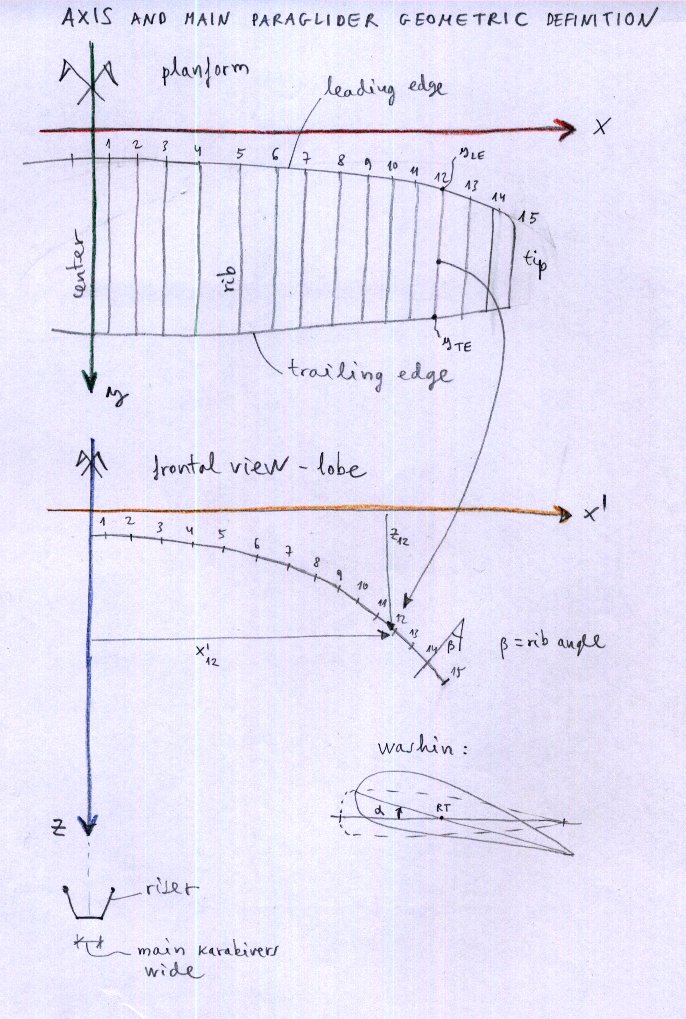
For each rib, and considering an orthonormal system of axes XYZ (Figure 4): X axis along the wingspan, Y axis along the central chord, Z axis vertical from the wing to the pilot.

Write in a horizontal line the following 11 parameters (parameters 10 and 11 are not mandatory):

  • integer : rib number
  • real : rib X coordinate
  • real : Y coordinate of the leading edge
  • real : Y coordinate of the trailing edge
  • real : X' coordinate of the rib in its final position in space
  • real : Z coordinate of the rib in its final position in space
  • real : angle "beta" of the rib to the vertical (degrees)
  • real : RP percentage of chord to be held on the relative torsion of the airfoils
  • real : washin in degrees defined manually (if parameter is set to "0")
  • real : angle of rotation of the profiles with respect to a vertical axis Z (degrees)
  • real : numeric value expressed as a percentage of the chord, where to place the vertical axis of rotation of the profiles

This is one of the most important parts of the wing definition process. These parameters can not be defined without a previous drawing, preferably in a CAD file, in which the desired plant is drawn to an appropriate scale, vault shape (wing arc), and inclination of the ribs on three axes. This drawing is one of the most basic and important design (pre‑process).

It would be possible to generate this drawing by a geometric preprocessor to read basic data from the wing desired number of cells, separation, size, shape, edge and trailing by a few parameters defined to create elliptical shapes. This optional pre‑processor has been implemented, but not inside the main program, because we prefer to keep this important part of design with a CAD program, to allow total freedom of the shape of the leading edge, trailing edge, and in the elevation, and inclination of the profiles. Any design is possible, normal wings, or bionic type, with peaks in leading edge or any other form. The pre‑processor is very useful and generates the geometry matrix that can be copied directly into this section. We are thinking about how to improve the pre‑processor to make it more intuitive, possibly with an html interface.

To define profiles at the center of the wing geometry, use the trick of defining a central cell of zero thickness.

washin

Figure 3. Washin


wing definition

Figure 4. Axis and main paraglider geometric design


rotated triangles

Figure 5. Only in "ss" paragliders, the parameter set to 0 or 1. If "1" then leading edge triangles will be no rotated. Control over specified ribs will be done using a real parameter 0.0 or 1.0 in last column of section 2, as explained below.

Note: Maximun allowed number of ribs is 100 per side (200 ribs or 199 cells).

SECTION 2: AIRFOILS

In an orderly manner for each rib, are written in a horizontal line:

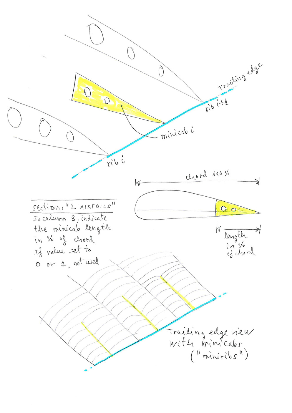
miniribs minicabs

Figure 6. Miribs definition in lep < 2.50 (since lep‑2.50 minirib "i" was defined at LEFT, between "i‑1" and "i")

Note: init and end points of the air openings are not fully implemented yet in the program, and is in the profile itself obliged to include it means of the integer numbers that describe the end of the top surface and the beginning of the intrados (in each airfoil).

MIDDLE UNLOADED RIBS: Added the possibility of using "middle unloaded ribs". Very easy to use: In section "2. AIRFOILS" at the last column use the parameter "100", means to place a complete unloaded rib in the middle of the panel, and the left corresponding rib. Similarly, as defined in the mini-ribs. But the parameter "100" activates a new specific programation. New plan numbered "1-6" with the new middle ribs numbered and marked. These ribs have been reformatted to achieve a perfect match with high precision, with the corresponding panels. In the center of the panels, are marked equidistant points in correspondence with the middle unloaded ribs. In addition, in the 2D-planform (plan "1-1"), also drawn in gray new ribs. Planned to draw in 3D (for reference) but not yet done. Important: To define holes in the ribs (elliptical or circles), add in section "4. AIRFOIL HOLES" a new hole type "11" that is defined exactly as the type "1" (hole type "1" and type "11" are exactly the same but the type "11" used exclusively by the middle unloaded ribs). In this case the initial rib number and end rib number with holes type "11" should be the same, and greater than the maximum number of ribs on one side, for example, use "50". See the attached example "leparagliding.txt". All new programation in section 9.9 of the source code.

- "Mini-ribs" are redefined, and now in section "2. AIRFOILS" at the last column, if you use the parameter "15", means to place a 15% mini-rib in the middle of the panel, and at the LEFT of the corresponding rib. Previously (lep < 2.50), mini-rib it was placed on the RIGHT. But it is better set at the left, so you can specify a minirib the center of the wing (Mini-rib specified in the left first rib). And this is consistent with the new middle unloaded ribs.

- Applied little optional displacement (to the center of the wing) in the points marking the position of the miniribs. Third parameter in the line of section "7. MARKS" of the datafile. Before, this displacement was set to default to zero.

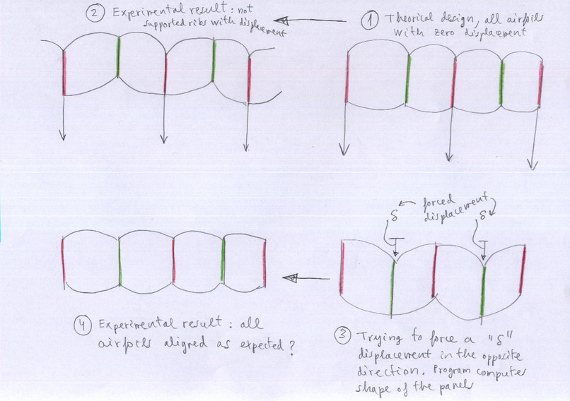
Delta displacement

Figure 7. Interpretation of parameter in sixth column. Parameter "delta" = forced displacement in cm of the rib perpendicular to the chord, and in the plane of the rib itself.

SECTION 3: ANCHOR POINTS

In an orderly manner for each rib, are shown in a horizontal line:

Note: A, B, C, D, E anchorages. F brakes.

SECTION 4: LIGHTENING IN THE RIBS (RIB HOLES)

By Rows:

Definition of each hole in a horizontal line. There are three possible types of holes. Type 1 = elliptical holes (including circulars), type 2 = elliptical holes central band, type 3 = triangular holes with smooth corners.

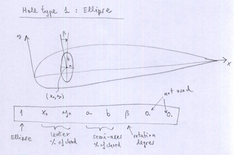
If the hole is type 1, type in a horizontal line:

hole 1

Figure 8. Hole type 1, ellipse

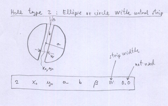
If the hole is type 2, type in a horizontal line:

Hole 2

Figure 9. Hole type 2, ellipse or circle with central strip

Not use holes type 2 because yet not implemented!

If the hole is type 3, type in a horizontal line:

hole 3

Figure 10. Hole type 3 triangle

If the hole is type 4, type in a horizontal line:

The main vertex or reference vertex of the rectangle is the bottom left. If the width value (a) is positive, the rectangle is drawn to the right of the main vertex. If the value of (a) is negative, then the rectangle is drawn to the left. Similar to the case of triangular holes.

Hole4

Image 10.1 Parameters for hole type 4 (rectangular)

Continue:

Definition of each hole in a horizontal line, as before.

And so on... (repeat pattern for all types of lightening configurations)

SECTION 5: SKIN TENSION

The tension of the top surface and lower surface panels is achieved by creating tapers in the panels. The program allows you to define "over‑wides" in 6 points along the edge of the panels. The transition between basis points of overwide is linear.

In each of the six lines are defined to indicate consecutively:

sk
A better explanation >
sk

Figure 11: Skin tension

Then add two more lines with the following parameter (new in leparagliding 2.0):

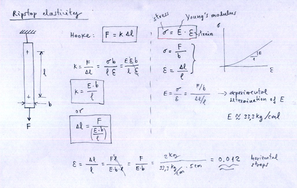
The justification for this value is obtained from the theory of elasticity. Leave the default value in case of doubt.

Ripstop elasticity

Figure 12. Ripstop elasticity

The justification for this line is complex. There are two possible interpretations:

First interpretation
If first number in NOT set to "1000", the values are used to make adjustments to the shape of the leading edge for easy sewing, using an "antiprecision" method. However is an old feature and actually is not recommended. Study conducted at the request of a manufacturer of paragliders. The second number is used to adjust the intensity of the modification (1.0=maximal effect, 0.0= no effect).

Justification of the line in the figure below:

sa

Figure 13. Sewing corrections

And the explanation:

When three panels are sewn at the same time, with different curvatures to side... problems may arise:

The left panel (i="izquierda") has a concave curvature, while the right panel (d="derecha") has a convex curvature.

The lengths of seam lines (line dashed) should be exactly the same. However, the outer edge of the fabric, which is 15 mm from the seam line, is shorter in the left case (inner radius) than the right (outer radius). The program calculates the difference in length of the leading edge in the area of "np" points of airfoil of greatest curvature from air inlet (np defined by user).

With the calculated length difference (1d2d‑1i2i), the program modifies the plan shape of the left panel, extending its inner side. Thus, when the seam is made, there are fewer problems ...

The second control parameter, "k" between 0. and 1. is the coefficient to be applied to the difference (1d2d‑1i2i). Then 0.0 = no effect. 1.0 = total effect. Then sewing corrections:

integer, real : Number of points np, k coefficient 0.0 to 1.0

Another explanation for the same, but in French: Étude des courbures panneaux‑nervures (PDF)

Many builders prefer not to take into account this effect, then select the parameter as k=0.0

Second interpretation Recommended for all designs

Set the parameters of the line to the values:

1000     1.0

First number "1000" (integer) is only a convention that signifies force the program to use maximal precision, reformatting panels to achieve accuracy better than 0.1 mm (lengths differences between rib and panels located at left and right).
Second number is a coefficient (real) between 0.0 and 1.0 that sets the intensity of the correction. If coefficient is set to "0.0" then is no correction. If the coefficient is set to "1.0" the accuracy is maximal, approx < 0.01 mm.

The description of the geometrical problem and the solution is described here.

In file lep‑out.txt is a report in section 6, indicating the final lengths of the panel at left, rib, panel at right, and maximal difference and distortions in mm.

SECTION 6: SEWING ALLOWANCES

SECTION 7: SEWING MARCAGE

Indicate the spacing in centimeters and the radius of the point, to make marks on ribs and panels to match all items as accurately and thus able to control that there is no slippage during sewing.

SECTION 8: ESTIMATING THE GENERAL ANGLE OF ATTACK

This section defines the basic length of the lines and provides the general draft of the wing, estimating the center of pressure and angle of glide.

Be entered on lines below:

calage

FIGURE 14: General AoA estimation

SECTION 9: DESCRIPTION OF LINES

We define the following concepts, per lines:

0 = lower branches lined only by geometric mean of the anchor points
1 = lower branches lined by weighting type 1
2 = lower branches lined by weighting type 2
3 = lower branches lined by weighting type 3 (spanwise and chordwise optimization). Read more details here.

Denotes the number of plans of lines that start from each of the risers of the glider. Will be considered as many plans as risers. The "plans" do not necessarily have lines in a plan, and may have different alignments anchors in various rows (pyramid lines).

(i1) number of branches (ramifications) of the path

(i2) branching level 1

(i3) order at level 1

(i4) level of ramification 2

(i5) order at level 2

(i6) level of ramification 3

(i7) order at level 3

(i8) branching level 4

(i9) order at level 4

(i10) anchor line (1 = A, 2 = B, 3 = C, 4 = C, 5 = D, 6 = brake)

(i11) anchor rib number

... and so on.

Do likewise with the other plans of the paraglider line design. The example of clear matrix writing is exposed in gnuLAB2 data file.

lines

FIGURE 15: Suspension lines matrix

SECTION 10: BRAKES

The first number is the length in cm for the main brake cable, and second number indicates the number of paths brake plane.

Matrix writes like for the rest of the lines, taking into account that now the level "1" corresponds to the main brake cable.

NOTE: i11 indicates rib number "i", where anchor the top line of the brakes. This number, usually an integer. Nevertheless, some versions ago was added an interesting feature. Is possible define a decimal which means the displacement of the anchoring point between the rib "i" and the rib "i+1". For example, 8.4 means anchor the line in the trailing edge, between rib 8 and 9, and 40% from the rib 8.

Brakes distribution:

brake distribution

Figure 16. Brake distribution

SECTION 11: RAMIFICATIONS LENGTH

Indicates the upper branch lengths to the anchors in sail, by rows:

ram

FIGURE 17: Ramifications length

SECTION 12: H V and VH RIBS

Then, for each mini‑rib, and in a row:

with the following meanings,

If it is a mini‑rib horizontal ribbon type:

Type 1: Horizontal strap between rib i1 and rib i2

1

Figure 18. Mini‑rib 1 (horizontal strap)

Type 2: Diagonal partial V‑rib centered in rib i

2

Figure 19. Mini‑rib 2 (V‑rib)

Type 3: Diagonal full V‑rib centered in rib i

3

Figure 20. Mini‑rib 3 (full V‑rib)

Type 4: "VH‑rib" between rib i‑1 to i+2

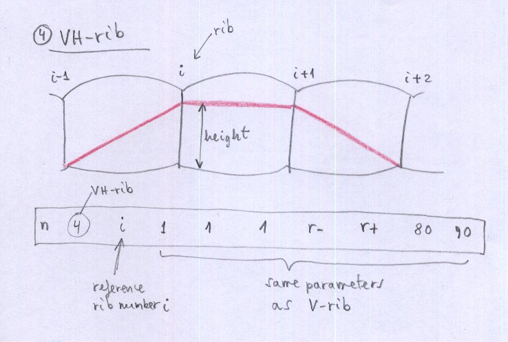
4

Figure 21. Mini‑rib 4 (VH‑rib)

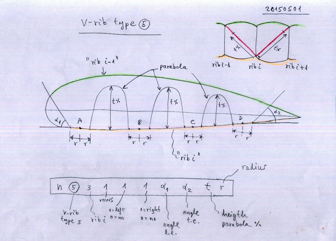
Type 5: full continuous VH‑rib centered in rib i

VRF

Figure 22. Full continuous V‑ribs type 5 using parabolic holes (if t<100%)

VRF

Figure 23. Full continuous V‑ribs type 5 using elliptical holes (if t>100%)

When using type 5 ribs keep in mind the following:
- The number of anchorages on the rib "i" must be equal to the number of anchors on the right and left, even if they are not used (they can be virtual, i.e. without lines)
- To define the Type 5 rib, use a number of lines equal to the number of anchors. Example:

1      5       5 1     1 1    60.0    60.0    80.     7.
2      5       5 2     1 1    60.0    60.0    80.     7.
3      5       5 3     1 1    60.0    60.0    80.     7.
4      5       5 4     1 1    60.0    60.0    80.     7.

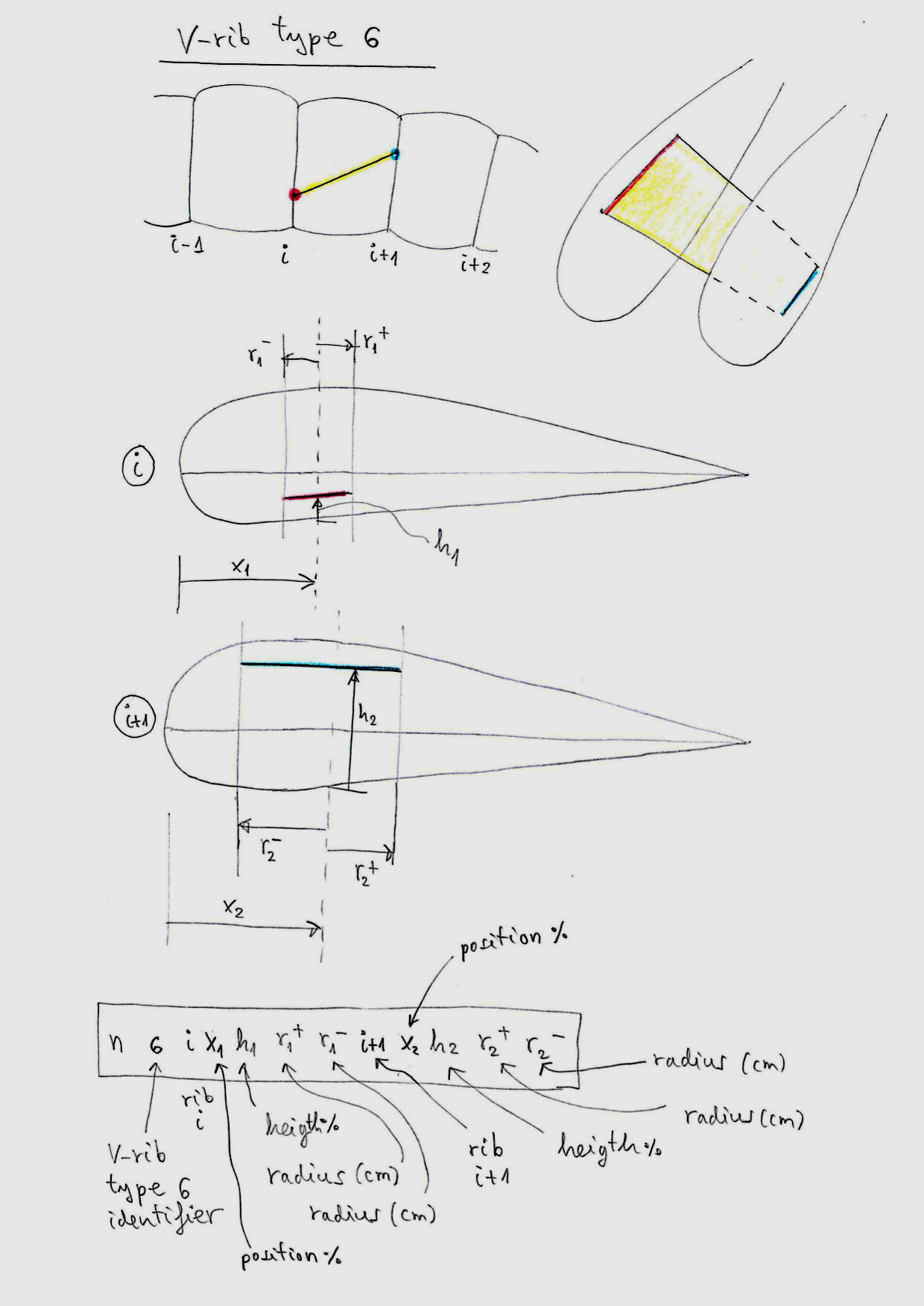
Type 6: general diagonal "VH‑rib" between rib i and rib i+1

Type 6 is a general diagonal. It's very simple. A trapezoidal diagonal ranging from rib number i to rib number i+1. But the rib is totally configurable in size and position. It has been designed to develop competition paragliders CCC types, which need to jump between 4 and 5 cells without lines. But it can also serve to design simplest paragliders, and replacing some of the types of diagonals described above. It is also very useful to define transverse horizontal strips located in all parts of the wing (the tapes have not necessarily coincide with the anchor points).

Type 6

Figure 24 V‑rib type 6 general diagonal

Parameters:

Type 6 uses 12 parameters, while the other V‑ribs types use only 10 parameters. This is no problem. The program can read the data file correctly. Simply, interpret the scheme. Try and see the results. Type‑6 is now working and fully implemented.

Very important:

The pieces "Type 6", must be defined consecutively, and line by line. With the following order: From the leading edge to the trailing edge, and from the center of the wing, to the wingtip. That is, first define all the pieces consecutively in rib number "i", before defining pieces in a rib greater than "i".

Ribs Types 11,12,13,14,15,16

Since version 3.14 of the program, six additional VH‑rib types can be used, named Type 11,12,13,14,15, and 16. Type 11 is the same as type 1, but absolute definitions of lengths in cm, now are set in % of the profile chord. The same for type 12 with respect to type 2, and so on until type 16, which is similar to type 6. Types 11 and 1, 12 and 2, 13 and 3, 14 and 4, cannot be combined in the same model. An auxiliary model can be made if necessary.

When you enter the settings to the types 1,2,3,4,5,6, the absolute lengths will be affected by the scaling factor of the wing (before this does not happen). This allows you to scale the wings more uniformly.

Since version 3.14 the graphical presentation of the VH‑ribs in 2D has been greatly improved, and ensuring that the reference decimal numbers are not shifted with respect to the pieces, as happened before. The roman numbers fit much better and its size may be defined in section 20.

Study examples, section 12 is very powerful and allows for almost any type of rib you can imagine. Example:

SECTION 12: H V and VH RIBS (exemple complet)

***************************************************
*   12. H V and VH ribs
***************************************************
24                                 > Use 24 VH-ribs
80    150                          > X Y spacing
1     11       0 1     1 1     3.5   0     0     0       > VH-rib 1, Type 11
2     11       1 1     2 1     3.5   0     0     0
3     11       2 1     3 1     3.5   0     0     0
4     11       3 1     4 1     3.5   0     0     0
5     11       8 4     9 4     6.0   0     0     0
6     12       3 3     1 1     3.0   7.0   80.   90.    > VH-rib 6, Type 12
7     12       5 3     1 1     3.0   7.0   80.   90.
8     12       7 3     1 1     3.0   7.0   80.   90.
9     12       9 3     1 1     3.0   7.0   80.   90.
10    13       2 4     1 1     3.0   10.0  0.    0.     > VH-rib 10, Type 13
11    13       4 4     1 1     3.0   10.0  0.    0.
12    13       6 4     1 1     3.0   10.0  0.    0.
13    14       2 2     1 1     3.0   7.0   80.   90.    > VH-rib 13, Type 14
14    14       5 2     1 1     3.0   7.0   80.   90.
15    14       8 2     1 1     3.0   7.0   80.   90.
16    14       11 2    1 1     3.0   7.0   80.   90.
17    15       3 1     1 1     60.   50.   81.   2.0    > VH-rib 17 to 20, Type 15
18    15       3 2     1 1     60.   50.   81.   2.0
19    15       3 3     1 1     60.   50.   81.   2.0
20    15       3 4     1 1     60.   50.   81.   2.0
21    16       10 80.  10.     3. 3. 11    75.   85. 8. 8.   > VH-rib 21, Type 16
22    16       11 75.  85.     8. 8. 12    75.   0.  3. 3.
23    16       6 18.   10.     3. 3. 7     18.   100. 5. 5.
24    16       7 18.   100.    5. 5. 8     18.   0.   3. 3.

Study examples, section 12 is very powerful and allows for almost any type of rib you can imagine.

SECTION 15: EXTRADOS COLORS

... and so on.

... and so on.

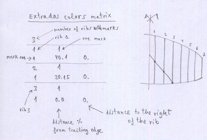
colors

Figure 25. Extrados colors

New method (since lep‑3.24) proposed by Pawel Lipsky (Altair Paragliders).

SECTION 15 Extrados colors and SECTION 16 Intrados colors.

It is now possible to define color cuts according to method "2":

Write by lines:

Example:

*****************************************************
*   15. Extrados colors
*****************************************************
-2
3
2   1
1   40.1   20.15   10.  0.
3   1
1   20.15   0.00   10.  0.
4   3
1       0.0    15.0   10.  0.
2       15.0   30.0   10.  0.
3       50.0   60.0   10.  0.

Same definition to define the intrados cuts (section 16).

Note: When the wing has an odd number of panels (center panel of nonzero width), the cut to the left of the center panel (panel 1) is defined exactly on the wing's axis of symmetry, for make symmetrical designs possible.

SECTION 16: INTRADOS COLORS

Like extrados colors, works from version >= 2.41. For example, you may write the minimal configuration:

1
1   1
1   0.    0.

SECTION 17: ADITIONAL RIB POINTS

With this option, auxiliary points can be drawn in the ribs. Typically to mark mylars, or start and end points of the nylon rods.

SECTION 18: ELASTIC LINES CORRECTION

Option to estimate the elastic elongation of the lines in normal flight configuration. These elongations are subtracted from strictly geometric length, so that in flight, are the exact lengths of project. Option fully functional but still under development. To calculate the elongation, we take into account the loads on each line, and the rigidity coefficient of each line, the elongation estimated by Hook's law: F = k·dx

This load distribution is also used when calculating line branches, optimized according to option number 3 (SECTION 9).

Example:

*****************************************************
*    18. Elastic lines corrections
*****************************************************
100
75   25               <<< A=75% B=25%
40   40   20          <<< A=40% B=40% C=20%
35   35   20   10     <<< A=35% B=35% C=20% D=10%
35   35   15   10   5 <<< A=35% B=35% C=15% D=10% E=5%
1   0.08   0.2   0.2
2   0.08   0.2   0.2
3   0.08   0.2   0.2
4   0.08   0.2   0.2
5   0.08   0.2   0.2

If you are using version until 2.60 of leparagliding, you do not need to continue typing, as it will not be considered. If you are using version 2.70 or higher, continue typing more settings.

SECTION 19: DXF LAYER NAMES

This section allows the user to choose some layers names in the DXF files. To facilitate the edition and modification of DXF files. In version 2.75 only the layers "points" "circles" and "triangles" are functional.

By lines, and regardless of the lines beginning with * which are comments or notes for help:

Line 1: integer – max layers number, now is 10.

Line 2: text1 text2
text1: general layer name (do not change this text)
text2: default layer name, to choose freely (with character and space restrictions)

Line 3: text1 text2
text1: line‑external (do not change this text)
text2: layer name for external cuts, to choose freely

Line 4: text1 text2
text1: line‑sewing (do not change this text)
text2: layer name for sewing lines, to choose freely

Line 5: text1 text2
text1: points (do not change this text)
text2: layer name for euclidean unidimensional points, to choose freely

Line 6: text1 text2
text1: circles (do not change this text)
text2: layer name for minicircle points, to choose freely. Minicircles as alternative for points.

Line 7: text1 text2
text1: triangles (do not change this text)
text2: layer name for minitriangles, to choose freely. Used is some special marks (tabs).

Line 8: text1 text2
text1: square (do not change this text)
text2: layer name for minisquares, to choose freely. Used is some special marks.

Line 9: text1 text2
text1: text (do not change this text)
text2: text layer name, to choose freely.

Line 10: text1 text2
text1: reference (do not change this text)
text2: reference layer name, to choose freely.

Line 11: text1 text2
text1: notes (do not change this text)
text2: notes layer name, to choose freely.

Example:

******************************************************
*    19. DXF layer names
******************************************************
10
general          default
line-external    cutexternal
line-sewing      cutinternal
points           points
circles          circles
triangles        triangle
square           square
text             text
reference        refer
notes            notes

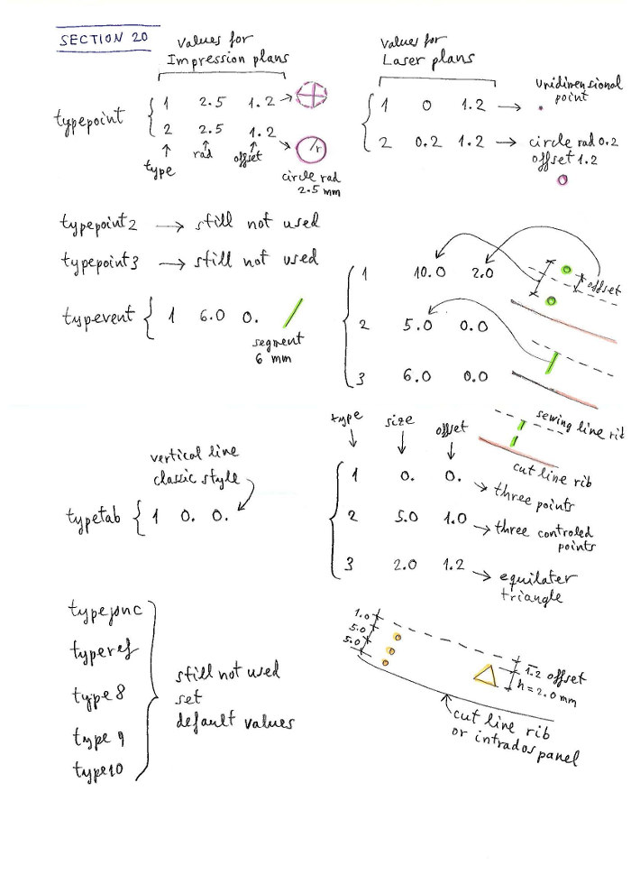
SECTION 20: MARKS TYPES

This section allows the user to choose different types of marking elements in DXF files (one‑dimensional points, minicircles, triangles, segments, ...). This is especially useful for laser cutting plotters, and the ability to adapt marking to manufacturer preferences. Remember that leparagliding generates two types of plans, some for use with conventional printer ("print" version), and others for professional use with computerized cutting plotters ("laser" version).

By lines, and regardless of the lines beginning with * which are comments or notes for help:

Line 1: integer – max number of different marks, now is 10.

Line 2 (typepoint – OK):
text integer real real integer real real
text: typepoint (point for general use)
integer: 1=constructed point, 2=minicircle – print
real: radius of minicircle in mm – print
real: offset in mm – print
integer: 1=unidimensional, 2=minicircle – laser
real: radius of minicircle in mm – laser
real: offset in mm – laser

Line 3 (typepoint2 – not used, set defaults):
text integer real real integer real real
text: typepoint2
integer: 1=unidimensional, 2=minicircle – print
real: radius in mm – print
real: offset in mm – print
integer: 1=unidimensional, 2=minicircle – laser
real: radius in mm – laser
real: offset in mm – laser

Line 4 (typepoint3 – not used, set defaults):
text integer real real integer real real

Line 5 (typevent – OK):
text integer real real integer real real
text: typevent
integer: 1=two green points, 2=segment, 3=double segment – print
real: points separation or segment in mm – print
real: offset in mm – print
integer: 1=two green points, 2=segment, 3=double segment – laser
real: points separation or segment in mm – laser
real: offset in mm – laser

Line 6 (typetab – OK):
text integer real real integer real real
text: typetab
integer: 1=three orange points, 2=three orange full control, 3=triangle – print
real: points separation or segment in mm – print
real: offset in mm – print
integer: 1=three orange points, 2=three orange full control, 3=triangle – laser
real: points separation or triangle height in mm – laser
real: offset in mm – laser

Line 7 (typejonc – not used, set defaults):
text integer real real integer real real
text: typejonc

Line 8 (typeref – not used, set defaults):
text integer real real integer real real
text: typeref

Line 9 (type8 – OK):
text integer real real integer real real
text: type8 – romano numbering in panels generated using section 29
integer: 1 not used
real: 0.2 spanning from 0.0 to 1.0 means the position of the roman number (0.0 totally to the left and 1.0 totally to the right, normal values 0.2 or 0.5) – print and laser
real: 4.0 means the vertical offset in mm with respect to the baseline. May be positive or negative number – print and laser
integer: 1 not used
real: 0.0 not used
real: 4.4 means the offset in mm between dots of the roman numeral (global size of the roman numerals) – print and laser

Line 10 (type9 – OK):
text integer real real integer real real
text: type9 – general numbers size, and roman marks size in ribs
integer: 1 not used
real: 0.0 not used
real: 7.0 decimal integer numbers size in cm, in leading edge, ribs, trailing edge panels
integer: 1 not used
real: 3.3 means the offset in mm between dots of the roman numeral (global size of the roman numerals) in rod pockets. If set to 0.0 then roman is not drawn – print and laser
real: 4.5 means the offset in mm between dots of the roman numeral (global size of the roman numerals) in ribs – print and laser

Line 11 (type10 – OK):
text integer real real integer real real
text: type10 – general numbers size in VH‑ribs, and roman marks size in VH‑ribs
integer: 1 not used
real: 0.0 not used
real: 6.0 decimal integer numbers size in cm, in VH‑ribs
integer: 1 not used
real: 0.0 not used
real: 4.5 means the offset in mm between dots of the roman numeral (global size of the roman numerals in VH‑ribs) – laser

S20

Figure 26a. Section 20 reference marks. Types 1,2,3,4,5,8,9,10 now fully functional.

S20 typm8

Figure 26b. Type8 marks parameters interpretation

Check that the parameters you use are correct, otherwise the size of the Roman numerals or decimals will not be appropriate. Since version 3.14 is VERY recommended to use this (or similar) example invariant bloc:

******************************************************
*    20. Marks types
******************************************************
10
typepoint  1 0.25 1.2    2 0.3 1.2
typepoint2 1 0.25 1.2    2 0.2 1.2
typepoint3 1 0.25 1.2    2 0.2 1.2
typevent   1 10.  0.0    2 2.0 0.0
typetab    1 10.  0.0    3 2.0 0.0
typejonc   1 10.  0.0    2 2.0 0.0
typeref    1 5.0  1.     1 2.0 0.0
type8      1 0.2  5.0    1 0.0 5.0
type9      1 0.0  7.0    1 3.2 4.5
type10     1 0.0  6.0    1 0.0 3.33

SECTION 21: JONCS DEFINITION (NYLON RODS)

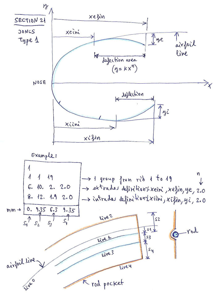
Section is fully functional. Now it is possible to define type 1 and type 2 rods, which are the most used. Type "1" is rod on the nose with small deflections at both ends, which are completely controllable in position, transition, and depth of deflection, with 8 parameters. Type "2" is straight or arched rod defined to any position within the profile, which can be at any position within the profile, defined by coordinates. The structure of the section is a bit complex, but it has its own logic. The program calculates the rods and shapes of the pockets, which are also fully controllable in widths, with 4 parameters. It is possible to define different rods for each cell, individually or by groups. If you don't need rods, leave the value to "0". In this section we will use the following basic concepts: scheme, bloc (of data), type (of rod), group (of ribs).

The first number in the section is an integer, which we called the "scheme".

The scheme "0" means, not defining any rod. And here ends the section. Easy!

Line 1: integer – if integer = 0 rods are not considered.

Example 1: Scheme "0" means do not use rods

*******************************************************
*    21. JONCS DEFINITION (NYLON RODS)
*******************************************************
0

The scheme "1" means use rods type "1" in the nose. At the bottom line write the number of groups. Then write each group consecutively using four lines. This is the detailed structure of the scheme 1:

Line 1: integer – if integer = 0 rods are not considered; if integer = 1 add some others parameters to define and draw rods.

Only if first integer is 1 (use joncs "type 1") then add:

Line 2: integer – number of groups to define.

Line 3: integer1 integer2 integer3
integer1: 1 (group number 1)
integer2: number of first rib in group 1
integer3: number of last rib in group 1

Line 4: real1 real2 real3 real4
real1: extrados init point deflection in % of chord
real2: extrados final point deflection in % of chord
real3: value of max deflection in intrados % of chord
real4: value n of exponent in curve of deflection type y=k·x^n (normally use n=2.0, parabolic)

Line 5: real1 real2 real3 real4
real1: intrados init point deflection in % of chord
real2: intrados final point deflection in % of chord
real3: value of max deflection in intrados % of chord
real4: value n of exponent in curve of deflection type y=k·x^n (normally use n=2.0, parabolic)

Line 6: real1 real2 real3 real4
real1: line 1, offset (mm) defining the rod (see figure)
real2: line 2, external width of pocket (mm)
real3: line 3, width for rod between sewing lines (mm)
real4: line 4, internal width of pocket (mm)

Lines 7,8,9,10 repeat same definitions for the group 2, and so on until final group.

Note that it is possible to define as many groups as profiles have the wing, and thus define a different rod for each profile. But normally with a group or two it is sufficient for the whole wing.

Example 2: Scheme "1". Using two groups. Group 1 from rib 1 to 15, and group 2 from rib 16 to 19.

*******************************************************
*    21. JONCS DEFINITION (NYLON RODS)
*******************************************************
1
2
1    1    15
2.0  1.0  3.0  2.5
3.0  2.0  4.0  2.0
2.0  5.0  3.0  2.0
2    16   19
2.0  1.0  3.0  2.5
3.0  2.0  4.0  2.0
2.0  5.0  3.0  2.0

Note: The parameters for type 2 rods (arched rods) are defined similarly but with a different structure. See the full manual for details.

SECTION 21: JONCS DEFINITION (NYLON RODS) – continuació

Example 2: Scheme "1". Using two groups. Group 1 from rib 1 to 15, and group 2 from rib 16 to 19.

*******************************************************
*    21. JONCS DEFINITION (NYLON RODS)
*******************************************************
1
2
1 1 15
5.5  10.    1.5   2.0
5.   11.    2.2   2.0
0.0  9.35  6.3   9.35
2    16 19
5.   9.     2.5   2.0
5.   12     3.    2.0
0.0  9.35  6.3   9.35
S21

Figure 27a. Section 21 joncs type 1 used in scheme "1"

The scheme "2":

Starting from version 3.12 of the program, the definition can be extended... :-) Now it is possible to define a more general model, called "scheme 2". In the scheme 2, we can add rods type "1" and many (not limited) rods type "2" within the profile. Type 2 are arc-shaped or straight-line rods. If deemed necessary, other types may be added later.

The structure is as follows:

Line 1: integer – integer: 2 means use scheme "2".

Line 2: integer – integer: number of data blocs to define.

Line 3: integer1 integer2
integer1: number of data bloc, starting with 1 and increasing by 1 the subsequent bloc
integer2: rod type can be 1, 2, or 3.

Line 4: integer – integer: number of groups to define.

If integer2 in line3 was 1, then write consecutively the four lines that define the geometry of the rods type 1 (lines 3,4,5,6 from scheme 1) and continue with more four lines for next group.

If integer2 in line3 was 2, then write consecutively the three lines that define the geometry of the rods type 2:

Rods type 2

Figure 27b. Rods type 2 (arch or straight line)

Line 5: integer1 integer2 integer3
integer1: 1 (group number 1)
integer2: number of first rib in group 1
integer3: number of last rib in group 1

Line 6: real1 real2 real3 real4 real5
real1: x‑coordinate of rod starting at point 1 (x1,y1) in % of airfoil chord
real2: y‑coordinate of rod starting at point 1 (x1,y1) in % of airfoil chord
real3: x‑coordinate of rod ending at point 2 (x2,y2) in % of airfoil chord
real4: y‑coordinate of rod ending at point 2 (x2,y2) in % of airfoil chord
real5: max deflection of the arc in % of airfoil chord. If 0.0 draws a straight line.

Line 7: real1 real2 real3 real4
real1: line 1, offset not used and put 0.0 value
real2: line 2, external width of pocket (mm)
real3: line 3, width for rod between sewing lines (mm)
real4: line 4, internal width of pocket (mm)

Continue with next group... Continue with next bloc of data...

If integer2 in line3 was 3, means use two rods per nose (upper and lower) for use in "shark nose" airfoils. Then write consecutively the following lines:

Line 4: integer – number of groups to define.

Line 5: integer1 integer2 integer3
integer1: 1 (group number 1)
integer2: number of first rib in group 1
integer3: number of last rib in group 1

Line 6: real1 real2 real3 real4 (same as rod type 1)
real1: extrados init point deflection in % of chord
real2: extrados final point deflection in % of chord
real3: value of max deflection in intrados % of chord
real4: value n of exponent in curve of deflection type y=k·x^n (normally use n=2.0, parabolic)

Line 7: real1 real2 real3 real4 (same as rod type 1)
real1: bottom part of upper rod init point deflection in % of chord
real2: parabolic deflection length in % of chord
real3: value of max deflection in % of chord
real4: value n of exponent in curve of deflection type y=k·x^n (normally use n=2.0, parabolic)

Line 8: real1 real2 real3 real4 (same as rod type 1)
real1: upper part of lower rod init point deflection in % of chord
real2: parabolic deflection length in % of chord
real3: value of max deflection in % of chord
real4: value n of exponent in curve of deflection type y=k·x^n (normally use n=2.0, parabolic)

Line 9: real1 real2 real3 real4 (same as rod type 1)
real1: intrados init point deflection in % of chord
real2: intrados final point deflection in % of chord
real3: value of max deflection in intrados % of chord
real4: value n of exponent in curve of deflection type y=k·x^n (normally use n=2.0, parabolic)

Line 10: real1 real2 real3 real4 (same as rod type 1)
real1: line 1, offset (mm) defining the rod (see figure)
real2: line 2, external width of pocket (mm)
real3: line 3, width for rod between sewing lines (mm)
real4: line 4, internal width of pocket (mm)

(continue same structure with next group if defined...)

View parameters interpretation:

S21.t3

Figure 27c. Rods type 3 definition (shark nose)

s21

Image double rod type 3 (shark nose)

If integer2 in line3 was 4, means use long extrados joncs. Then write consecutively the following lines:

Line 4: integer – number of groups to define.

Line 5: integer1 integer2 integer3
integer1: 1 (group number 1)
integer2: number of first rib in group 1
integer3: number of last rib in group 1

Line 6: real1 real2 real3 real4
real1: extrados init point deflection in % of chord
real2: extrados final point deflection in % of chord
real3: value of max deflection in intrados % of chord
real4: value n of exponent in curve of deflection type y=k·x^n (normally use n=2.0, parabolic)

Line 7: real1 real2 real3 real4
real1: extrados init point deflection in % of chord
real2: extrados final point deflection in % of chord
real3: value of max deflection in intrados % of chord
real4: value n of exponent in curve of deflection type y=k·x^n (normally use n=2.0, parabolic)

(continue same structure with next group if defined...)

If integer2 in line3 was 5, means use long intrados joncs. Then write consecutively the following lines:

Line 4: integer – number of groups to define.

Line 5: integer1 integer2 integer3
integer1: 1 (group number 1)
integer2: number of first rib in group 1
integer3: number of last rib in group 1

Line 6: real1 real2 real3 real4
real1: extrados init point deflection in % of chord
real2: extrados final point deflection in % of chord
real3: value of max deflection in intrados % of chord
real4: value n of exponent in curve of deflection type y=k·x^n (normally use n=2.0, parabolic)

Line 7: real1 real2 real3 real4
real1: extrados init point deflection in % of chord
real2: extrados final point deflection in % of chord
real3: value of max deflection in intrados % of chord
real4: value n of exponent in curve of deflection type y=k·x^n (normally use n=2.0, parabolic)

(continue same structure with next group if defined...)

s21

Rods type 1 (nose), type 4 (extrados), and type 5 (intrados)

This definition may seem complicated (and it is!) but is understood better with examples and doing tests and seeing the results.

Example 3: Commented scheme "2". Using only one data bloc type 2 and two groups. Group 1 from rib 1 to 15, and group 2 from rib 16 to 19.

*******************************************************
*    21. JONCS DEFINITION (NYLON RODS)
*******************************************************
2                      < scheme 2
1                      < only one bloc
1 2                    < bloc 1 uses rods type 2
2                      < bloc 1 uses two groups
1 1 15                 < group 1 from rib 1 to 15
20. 2.  30. -2.0 3.0   < coordinates (x1,y1) (x2,y2) and deflection all in % of chord
0.0  9.35  6.3  9.35   < rod pocket sizes in mm
2 16 20                < group 2 from rib 16 to 20
40. 4.  30. -3.2 0.0   < coordinates (x1,y1) (x2,y2) and deflection all in % of chord
0.0  9.35  6.3  9.35   < rod pocket sizes in mm

Example 4: Commented scheme "2". Using two data blocs and two groups in each bloc.

*******************************************************
*    21. JONCS DEFINITION (NYLON RODS)
*******************************************************
2                      < scheme 2
2                      < use two blocs
1 1                    < first bloc uses rods type 1
2                      < first bloc uses two groups
1 1 15                 < group 1 from rib 1 to 15
5.5  10.   1.5   2.0
5.   11.   2.2   2.0
0.0  9.35  6.3   9.35
2    16 19              < group 2 from rib 16 to 20
5.   9.    2.5   2.0
5.   12    3.    2.0
0.0  9.35  6.3   9.35
2 2                    < second bloc uses rods type 2
2                      < second bloc uses two groups
1 1 15                 < group 1 from rib 1 to 15
20. 2.  30. -2.0 3.0   < coordinates (x1,y1) (x2,y2) and deflection all in % of chord
0.0  9.35  6.3  9.35   < rod pocket sizes in mm
2 16 20                < group 2 from rib 16 to 20
40. 4.  30. -3.2 0.0   < coordinates (x1,y1) (x2,y2) and deflection all in % of chord
0.0  9.35  6.3  9.35   < rod pocket sizes in mm

Example 5: Scheme "2" using one data bloc, first data bloc type 3 "shark nose", one group from rib 1 to 30.

*******************************************************
*    21. JONCS DEFINITION (NYLON RODS)
*******************************************************
2                      < scheme 2
1                      < one bloc
1 3                    < first bloc type 3 "shark nose"
1                      < one group
1 1 30                 < first group from rib 1 to 30
4.2   10.8    1.0   2.0  < coordinates (x1,y1) (x2,y2) and deflection all in % of chord
3.5   5.0     1.0   0.7  < upper rod initial point % of parabolic modification, length, deflection, exponent
4.5   5.0     2.2   1.0  < upper rod initial point % of parabolic modification, length, deflection, exponent
3.67  12.1    0.79  2.0  < coordinates (x1,y1) (x2,y2) and deflection all in % of chord
0.0   10.35   6.3   9.35 < rod pocket sizes in mm

Number of data blocs limited to 20, and number of groups to 100, then a lot of rods in each airfoil! Test and see the results!

S21

Figure 27c. Rods type 1 (nose reinforcement) and type 2 (arch or straight line)

Example 6: using rods type 1, 2, 4:

*******************************************************
*    21. JONCS DEFINITION (NYLON RODS)
*******************************************************
2                > Scheme 3
3                > Use 3 blocks
1 1              > Block 1 type 1
1
1 1 25
12.0  18.5     1.5   2.0
7.0   15.0     2.0   2.0
0.0    9.35    6.3   9.35
2 4              > Block 2 type 4
1
1 1 25
23.5  29.5   1.1   2.0
63.0  70.0   1.1   2.0
0.0    9.35  6.3   9.35
3 5              > Block 3 type 5
1
1 1 25
23.5  29.5   1.1   2.0
63.0  70.0   1.1   2.0
0.0    9.35  6.3   9.35

SECTION 22: NOSE MYLARS DEFINITION

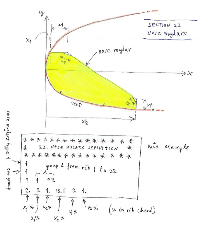
This section allows the user to draw nose mylars.

Line 1: integer
if integer = 0 mylars are not considered
if integer = 1 add some others parameters to define and draw mylars

Example 1:

*******************************************************
*    22. NOSE MYLARS DEFINITION
*******************************************************
0

Example 2:

*******************************************************
*    22. NOSE MYLARS DEFINITION
*******************************************************
1
1
1    1    22
2.   3.0   1.0   13.5   3.   1.
S22

Figure 28. Section 22 nose mylars definition

SECTION 23: TAB REINFORCEMENTS

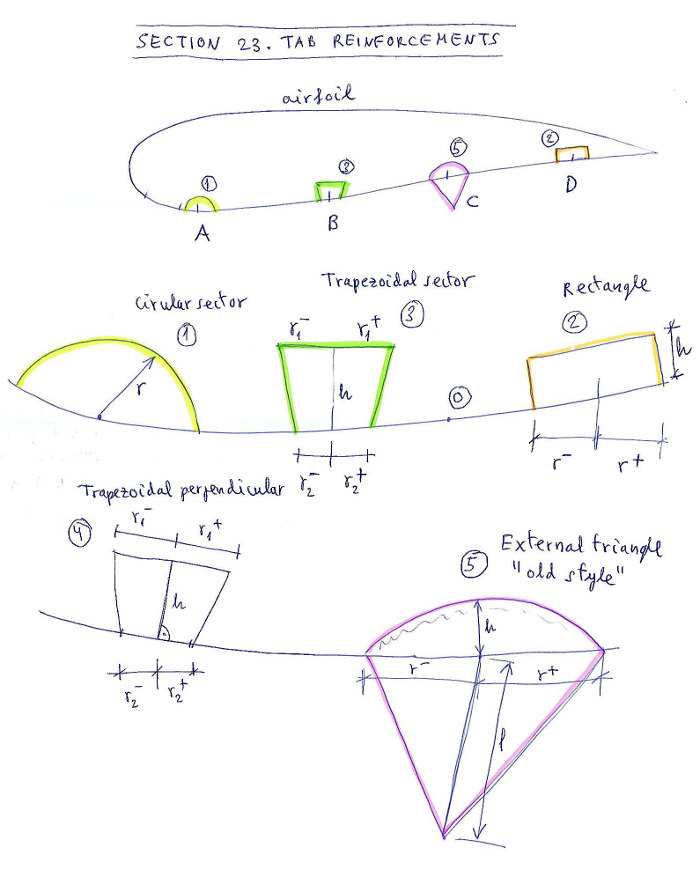
This section allows the user to draw tab reinforcements. Still not functional. Leave the value to "0".

Line 1: integer
if integer = 0 tab reinforcements are not considered
if integer = 1 add some others parameters to define tab reinforcements

Example 1:

*******************************************************
*    23. TAB REINFORCEMENTS
*******************************************************
0

Example 2:

*******************************************************
*    23. TAB REINFORCEMENTS
*******************************************************
1
1
1  1  22
2  2  1  5  3
schemes
1  0    p1   p2   p3   p4   p5
2  0    p1   p2   p3   p4   p5
3  0    p1   p2   p3   p4   p5
4  1    p1   p2   p3   p4   p5
5  1    p1   p2   p3   p4   p5

In this data, one group of reinforcements applicable to ribs 1 to 22 is defined. On the tabs A B C D E, the "schemes" 2,2,1,5,3 respectively are applied. The schemes are defined below the word "schemes":

S23

Figure 29. Section 23 tab reinforcements

Another example, with two groups: group 1 from ribs 1 to 10, group 2 from 11 to 22. Group 2 uses scheme "1" for all tabs.

*******************************************************
*    23. TAB REINFORCEMENTS
*******************************************************
1
2
1  1  10
2  2  1  5  3
2  11  22
1  1  1  1  1
schemes
1  0    p1   p2   p3   p4   p5
2  0    p1   p2   p3   p4   p5
3  0    p1   p2   p3   p4   p5
4  0    p1   p2   p3   p4   p5
5  1    p1   p2   p3   p4   p5

SECTION 24: GENERAL 2D DXF OPTIONS

This section allows the user to define some colors in the 2D DXF plans.

Line 1: integer
if integer = 0 DXF options set by default
if integer = 1 add some others parameters for DXF

Only if first integer is 1 then add:

Line 2: text1 integer text2
text1: A_lines_color (do not change this text)
integer: color number index for "A" lines
text2: color name (optional text not used)

Line 3: text1 integer text2
text1: B_lines_color (do not change this text)
integer: color number index for "B" lines
text2: color name (optional text not used)

Line 4: text1 integer text2
text1: C_lines_color (do not change this text)
integer: color number index for "C" lines
text2: color name (optional text not used)

Line 5: text1 integer text2
text1: D_lines_color (do not change this text)
integer: color number index for "D" lines
text2: color name (optional text not used)

Line 6: text1 integer text2
text1: E_lines_color (do not change this text)
integer: color number index for "E" lines
text2: color name (optional text not used)

Line 7: text1 integer text2
text1: F_lines_color (do not change this text)
integer: color number index for "F" brake lines
text2: color name (optional text not used)

Example:

*******************************************************
*    24. GENERAL 2D DXF OPTIONS
*******************************************************
1
A_lines_color    1    red
B_lines_color    30   orange
C_lines_color    3    green
D_lines_color    4    cyan
E_lines_color    6    magenta
F_lines_color    5    blue

Note: Remember usual color index numbers for CAD systems: 1=red, 2=yellow, 3=green, 4=cyan, 5=blue, 6=magenta, 7=white, 8=dark grey, 9=grey, ... up to 255 depending on your color palette. It is preferable not to use colors with more than two digits.

SECTION 25: GENERAL 3D DXF OPTIONS

This section allows the user to define some colors in the 3D DXF plans. Allows to draw unifilar not ovalized versions of the surfaces.

Line 1: integer
if integer = 0 DXF options set by default
if integer = 1 add some others parameters for the 3D DXF

Only if first integer is 1 then add:

Line 2: text1 integer text2
text1: A_lines_color (do not change this text)
integer: color number index for "A" lines
text2: color name (optional text not used)

Line 3: text1 integer text2
text1: B_lines_color (do not change this text)
integer: color number index for "B" lines
text2: color name (optional text not used)

Line 4: text1 integer text2
text1: C_lines_color (do not change this text)
integer: color number index for "C" lines
text2: color name (optional text not used)

Line 5: text1 integer text2
text1: D_lines_color (do not change this text)
integer: color number index for "D" lines
text2: color name (optional text not used)

Line 6: text1 integer text2
text1: E_lines_color (do not change this text)
integer: color number index for "E" lines
text2: color name (optional text not used)

Line 7: text1 integer text2
text1: F_lines_color (do not change this text)
integer: color number index for "F" brake lines
text2: color name (optional text not used)

Line 8: text1 integer integer text2
text1: Extrados (do not change this text)
integer: if set to "0" unifilar extrados is not drawn, if set to "1" is drawn
integer: color index for the extrados
text2: optional text with the color name

Line 9: text1 integer integer text2
text1: Vents (do not change this text)
integer: if set to "0" unifilar vents is not drawn, if set to "1" is drawn
integer: color index for the vents
text2: optional text with the color name

Line 10: text1 integer integer text2
text1: Intrados (do not change this text)
integer: if set to "0" unifilar intrados is not drawn, if set to "1" is drawn
integer: color index for the intrados
text2: optional text with the color name

Example:

*******************************************************
*    25. GENERAL 3D DXF OPTIONS
*******************************************************
1
A_lines_color    1    red
B_lines_color    8    grey
C_lines_color    8    grey
D_lines_color    8    grey
E_lines_color    8    grey
F_lines_color    30   orange
Extrados    1    5    blue
Vents       0    1    red
Intrados    1    3    green

SECTION 26: GLUE VENTS

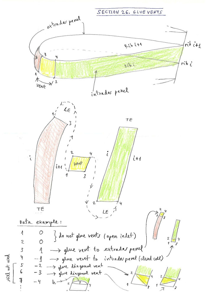
This section allows us to define different types of air inlets (vents), and automatically "glue" into the panel of extrados, intrados, or to separate them. The vents include sewing edges. The skin tension in the vent is linear and automatically corresponds to that defined at the points corresponding in extrados and intrados.

The vent definition is very easy and intuitive. A row is defined for each rib. The first number is the rib number, the next is the vent type, and then zero, two, or three parameters, depending on the type.

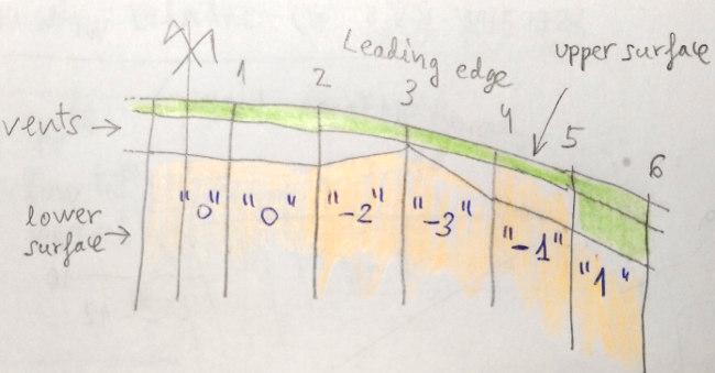
Available vent types (version lep‑3.17) 0,1,-1,-2,-3,4,-4,5,-5,6,-6:

Section 26 structure:

Line 1: integer
if integer = 0 then end the section and use old vents style (not recommended)
if integer = 1 add some others parameters for precise vents control.

Only if first integer is 1 then add N lines, one for each airfoil number i:

Line i: integer1 integer2 real1 real2 real3
integer1: airfoil number (cell between airfoil i and airfoil i‑1)
integer2: vent parameter (available parameters 0, 1, -1, -2, -3, 4, -4, 5, -5, 6, -6 as explained above)
real1: parameter 1 (0 to 100). Start point at left (vents 4, -4, 5, -5), or horizontal axis in 6, -6
real2: parameter 2 (0 to 100). Start point at right (vents 4, -4, 5, -5), or vertical axis in 6, -6
real3: parameter 3 (0 to 100). Arch depth in vents type 5 or -5

Example 1 (use old style, not recommended):

*******************************************************
*    26. GLUE VENTS
*******************************************************
0

Example 2 (full vent control):

*******************************************************
*    26. GLUE VENTS
*******************************************************
1
1    0
2    0
3    1
4   -2
5   -3
...
20  -2
21  -1
22  -1
23  -1

Example 3 (advanced vents):

*******************************************************
*    26. GLUE VENTS
*******************************************************
1
1    0
2    0
3    1
4   -4 100. 0.   ---> general diagonal vent from 100% to 0%
5   -4 10. 50.   ---> general diagonal vent from 10% to 50%
...
19  -5 0. 0. 15  ---> arc vent 15% depth
20  -6 80 80     ---> elliptical inlet
21  -1
22  -1
23  -1
S26

Figure 30. Glue vents

vents types

Figure 31: Vents types 0,1,-1,-2,-3

Vents 4,-4,5,-5,6,-6

Figure 31b: Vents types -4,4 (general diagonal) -5,5 (general arc) -6,6 (elliptical inlet), available in lep‑3.17 and later. Note that type 4 also includes cases 0,1,2,3, and type -4 cases 0, -1, -2, -3. Finally type 5 includes case 4, and -5 includes case -4.

SECTION 27: SPECIAL WINGTIPS

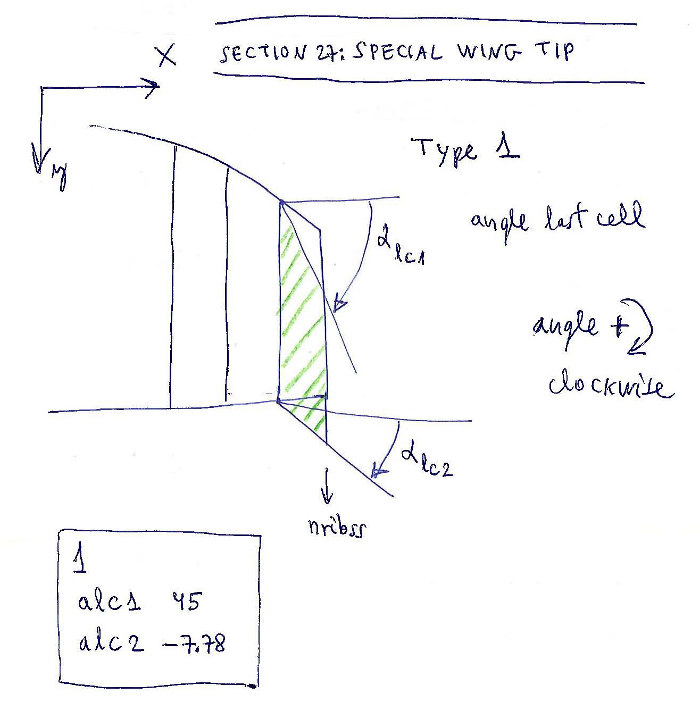
It is used for defining wingtips with special shapes. Available values 0, 1, 2.

Wingtip type "1":

Section 27

Figure 32. Special wingtip

Line 1: integer
if integer = 0 do not add wingtip modifications (set by default)
if integer = 1 add some wingtip modifications.

Only if first integer is 1 then add:

Line 2: text real
text: AngleLE (do not change this text)
real: angle in degrees between the horizontal and the leading edge in the last cell.

Line 3: text real
text: AngleTE (do not change this text)
real: angle in degrees between the horizontal and the trailing edge in the last cell.

Example 1:

*******************************************************
*    27. SPECIAL WING TIP
*******************************************************
1
AngleLE 45
AngleTE -7.78

"1" refers to define "type 1" wing tip modifications. It is planned to define several modifications. Type 1 is the simplest. "AngleLE" is a name not computed. It serves to remember that next we have to write the new angle in degrees between the horizontal and the leading edge in the last cell. It is usual to force the angle of the last cell, and this section allows it to be done without modifying the geometry matrix. Set 45° for example. "AngleTE" is a name not computed for the trailing edge. Set the angle as desired, -7.78° for example.

Example 2:

*******************************************************
*    27. SPECIAL WING TIP
*******************************************************
0

Wingtip type "2":

In 3.27+ version, I have started working on the rounded wingtip with a parabola, but only draw in planform, not redesign the panels yet :( Read more: https://laboratoridenvol.com/leparagliding/dev/lep-dev.en.html

Example, special wingtip type 2:

*******************************************************
*    27. SPECIAL WING TIP
*******************************************************
2
AngleLE 45
AngleTE -7.78

SECTION 27: SPECIAL WINGTIPS – continuació

Example, special wingtip type 2 (rounded wingtip with parabola):

*******************************************************
*    27. SPECIAL WING TIP
*******************************************************
2
Distance  60.
Angle     0.

SECTION 28: PARAMETERS FOR CALAGE VARIATION

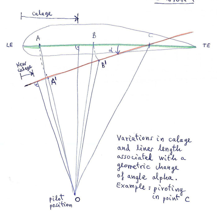
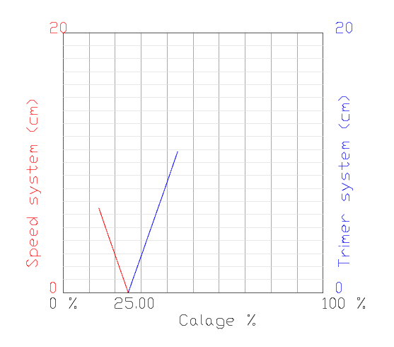
Study the variations in the riser lengths and calage when applying speed system or trim system. It is interesting to experiment with new calages in prototypes or to define the speed or trim systems.

s28a

Figure 33. Principles of the study of the calage variations.

We study the variations in the riser lengths when applying accelerator (speed system) pivoting in the last riser (most common case), which remains with constant length. For practical purposes we define a negative alpha angle of pitch increased in N1 spaces gradually, and then we compute the variations in the line lengths and calage. We do the same study, assuming a trim system that increases the pitch angle in N2 spaces gradually. In this case, the most usual is to consider the constant length A riser and the other variables in length.

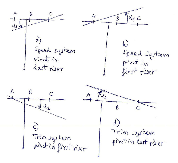
The program analyzes a total of 4 cases, depending on the pivot point and if it is reduction or increase in angle:

s28b

Figure 34. Cases a,b,c,d reported in file lep-out.txt

In output file SECTION 7: lep-out.txt we see the tables that relate in detail the variations of angle, with the calage variations, and increments or decrements of length in each riser. It is interesting to experiment with new calages in prototypes or to define the speed or trim systems. Four cases:

Example lep-out.txt:

a) Speed system pivot in last riser:
-------------------------------------------
 i   alpha       A       B       C    Calage
 1     .00     .00     .00     .00   25.00
 2   -1.00   -2.18   -1.29     .00   21.19
 3   -2.00   -4.35   -2.59     .00   17.40
 4   -3.00   -6.52   -3.88     .00   13.66

Write data in SECTION 28 with one or four lines:

Line 1: integer
if integer = 0 do nothing
if integer = 1 do calage study "type 1".

Only if first integer is 1 then add:

Line 2: integer – number of risers to be considered (2,3,4,5 or 6).

Line 3: real1 real2 real3 real4 real5 real6
real1: % of central chord for riser A (is not necessary to match anchor position)
...
real6: % of central chord for riser E (is not necessary to match anchor position).

Line 4: real1 integer1 real2 integer2
real1: max angle (negative) in degrees set by the speed system
integer1: number of steps in angle for study purpose
real2: max angle (positive) in degrees set by the trim system
integer2: number of steps in angle for study purpose.

Example:

*******************************************************
*    28. PARAMETERS FOR CALAGE VARIATION
*******************************************************
1
3
10. 30.35  60  0  0  0
-4 4 5 10

Explanation:

s28c

Figure 35. New graphic in plan 2-1 (.dxf output)

SECTION 29: 3D SHAPING

The model of 3D-Shaping proposed by the Laboratori, consists in making one or two transverse cuts in the upper surface, near the leading edge, and another optional cut on the bottom surface. We will call this model as "type 1". The edges of the transverse cuts will be modified from the straight line into an arc of a circle. In this way, we can "add fabric" lengthwise and we can control the ovalization and the tension in this direction. Ovalization in transverse direction is achieved via the module of skin tension (SECTIONS 5 or 31). In summary, we can control the amount of tissue and tension in transverse and in longitudinal direction near the nose, where the curvatures are greatest.

To set the parameters of the 3D-shaping in the model "type 1" is necessary to study the profile in detail, viewing and counting the individual points that form it, Laboratori style! :-) You need to view your profile in CAD (or in the .txt file), identify and count points. Remember that the points in a profile are counted starting in the trailing edge (point 1), continuing by the upper surface, nose, vents, lower surface, and ending again in the trailing edge. Exactly as described previously. We could define another model "type 2" where the position of the cut points are defined in % of the length of the panel, but in this model 1, is considered to specify exactly the points considered.
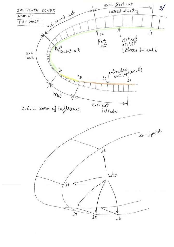
For each cut, it is necessary to define a "zone of influence". In the zones of influence is measured the length of a section of the profile and is compared with the corresponding length in the ovalized profile. This question is fundamental to understand the 3D-shaping type 1. It is necessary to view the figure below:

3d

Figure 36. Cuts and zones of influence. J1,j2,j3,j4,j5,j6,j7 indicate numeric values of the selected points in the profile, starting to count from the trailing edge. J4 and j5 are the vent points.

For the purposes of notation, we will call the different parts in which we divide the profile as:

In each zone 1,2,3,4,5,6 the program computes the length of the arch of airfoil (d1) and the arch of the ovalized airfoil (d2). The differences of longitude (d2-d1) are calculated automatically in each zone, and then applied consistently to each cut with a value (f) obtained using the values (d2-d1) of the adjacent zones. Is provided a setting parameter around 1.0, which serves the designer to regulate the depth of the 3D-shaping in each cut (positive or negative), in relation to the automatic calculation. Thus, using the coefficient of 1.0, the depth of 3D is according to the theory exposed. Using a coefficient of 0.0 does not apply the 3D effect, and using values higher or lower than 1.0 increases or decreases the effect. The control of the depth of 3D-shaping is continuous and individual for each cut. A more detailed description, and the formulas used in the calculation are described in this technical note about 3D-shaping. For each rib, a full report of the values d1, d2, d2-d1, computed in each zone, and the final values f applied in each cut are printed in tabular form in section 9 of the file lep-out.txt.

Also, for verification purposes, a new section 10 is written to the lep-out.txt file with the counting of the points of each profile, to verify that they are all the same for all profiles, and that they are compatible with the defined cuts.

It should be noted, that the parameters applied in this section, will be usually "invariant values" applied to the majority of the designs. We just have to think about all this, a single time for each type of profile. And the Laboratory will provide soon the recommended values in next designs. Of course, finding the good parameters is a real art. The program LEparagliding now provides the tools to make numerical and graphical experiments (lep-out.txt section 9 and leparagliding.dxf plan in box 1-8).

Negative 3D-shaping values are available since version 3.11.

Explanation of the parameters in SECTION 29:

Line 1: integer
if integer = 0 then do not use 3D-shaping, and finish writing the section.
if integer = 1 then use 3D-shaping, and continue writing.

Line 2: integer – type of 3D-shaping theory used, now we use only model "type 1" using transverse cuts, set parameter to 1.

Line 3: character integer
character = groups
integer = number of groups used.

Line 4: character integer1 integer2 integer3
character = group
integer1 = number of the group
integer2 = initial rib in group
integer3 = final rib in group.

Line 5: character integer1 integer2
character = upper, word meaning upper surface (extrados)
integer1 = number of cuts in upper surface (possible values 1 or 2)
integer2 = subtype of cuts, set to 1, only value accepted.

Line 6: integer1 integer2 real
integer1 = initial point in the first zone of influence (j1)
integer2 = point where the first cut is set (j2)
real = "depth" of 3D-shaping in the cut, possible values -1.0, -0.4, 0.0, 0.1, ..., 1.0, 1.2, ... (multiplier coefficient around ±1.0).

Line 7: integer1 integer2 real (only if we use two extrados cuts)
integer1 = initial point in the second zone of influence (j2)
integer2 = point where the second cut is set (j3)
real = "depth" of 3D-shaping in the cut, possible values -1.0, -0.4, 0.0, 0.1, ..., 1.0, 1.2, ...

Line 8: character integer1 integer2
character = lower, word meaning lower surface (intrados)
integer1 = number of cuts in lower surface (possible values 0 or 1)
integer2 = subtype of cuts, set to 1, only value accepted.

If the number of cuts in intrados is 0, stop writing, else:

Line 9: integer1 integer2 real
integer1 = point where the intrados cut is set (j6)
integer2 = final point in the intrados zone of influence (j7)
real = "depth" of 3D-shaping in the cut, possible values -1.0, -0.4, 0.0, 0.1, ..., 1.0, 1.2, ...

(...Repeat lines 5,6,7,8,9 for next groups...)

Line 10: character – character = "* print parameters:" (comment line, it is mandatory to write something).

Line 11: character integer1 integer2 integer3 integer4
character = Inter3D, word to indicate representation of the intermediate airfoils in 3D lep-3d.dxf
integer1 = 0 indicates do not draw, and 1 draw
integer2 = index of first airfoil to draw
integer3 = index of last airfoil to draw
integer4 = 0 indicates to draw with symmetry, 1 only one side.

Line 12: character integer1 integer2 integer3 integer4
character = Ovali3D, word to indicate representation of the intermediate ovalized airfoils in 3D lep-3d.dxf
integer1 = 0 indicates do not draw, and 1 draw
integer2 = index of first airfoil to draw
integer3 = index of last airfoil to draw
integer4 = 0 indicates to draw with symmetry, 1 only one side.

Line 13: character integer1 integer2 integer3 integer4
character = tesse3D, word to indicate representation of panel tessellation in 3D lep-3d.dxf
integer1 = 0 indicates do not draw, and 1 draw
integer2 = index of first panel to draw
integer3 = index of last panel to draw
integer4 = 0 indicates to draw with symmetry, 1 only one side.

Line 14: character integer1 integer2 integer3 integer4
character = exteDXF, word to indicate representation of panels tessellation in 3D in a new external DXF file (possible use in CFD analysis)
integer1 = 0 indicates do not draw, and 1 draw
integer2 = index of first panel to draw
integer3 = index of last panel to draw
integer4 = 0 indicates to draw with symmetry, 1 only one side.

Line 15: character integer1 integer2 integer3 integer4
character = exteSTL, word to indicate representation of panels tessellation in 3D in a new external STL file (used with programs of 3D modelling as OpenSCAD or FreeCAD)
integer1 = 0 indicates do not draw, and 1 draw
integer2 = index of first panel to draw
integer3 = index of last panel to draw
integer4 = 0 indicates to draw with symmetry, 1 only one side.

Important: If section 29 is not "0" then lines 12, 13, 14, 15 are mandatory to write. Since lep‑3.19 the actions are fully functional. These parameters will generate independent dxf files with the ovalized surfaces, and even a .stl model to view with FreeCAD or OpenSCAD, or even analyze with CFD programs.

All this may seem complicated, but it is much easier to understand section structure watching a few examples:

Example 1: Do not use 3D-shaping. Set one line with "0" parameter and stop writing. It is the simplest solution to avoid the complicated 3D-shaping module! :)

*******************************************************
*    29. 3D SHAPING
*******************************************************
0

Example 2: Active 3D-shaping module but without any cut. The utility of defining this, is that the representation of plan 1-8 is activated automatically, with the drawing of the intermediate and ovalized airfoils in 2D. You can also activate the 3D representations in 3D, changing the settings "0" to "1" in the "Print parameters" subsection. In general, preferable to use example 2, than example 1 (the two are invariant sections).

************************************************************
*    29. 3D SHAPING
************************************************************
1
1
groups  1
group   1    1    1
upper   0    1
lower   0    1
* Print parameters
Inter3D 0    1    1    0
Ovali3D 0    1    1    0
tesse3D 0    1    1    0
exteDXF 0    1    1    0
exteSTL 0    1    1    0

Example 3: Easy case, only one group and one cut in extrados. First group from rib 1 to 14 using one cut type 1 in upper surface and zero in lower surface. Zone of influence of first cut started in point 30 and cut located in point 40, depth of the effect 0.8. Zero cuts in lower surface, type 1. Prints 3D intermediate (Inter3D) and ovalized (Ovali3D) airfoils at the left of ribs 1 to 14.

*******************************************************
*    29. 3D SHAPING
*******************************************************
1
1
groups  1
group   1    1    14
upper   1    1
1       30   40   0.8
lower   0    1
* Print parameters
Inter3D 1    1    14   0
Ovali3D 1    1    14   0
tesse3D 0    1    1    0
exteDXF 0    1    1    0
exteSTL 0    1    1    0

Example 4: General case, using two groups. First group from rib 1 to 10 using two cuts in upper surface and one in lower surface. Zone of influence of first cut started in point 25 and cut located in point 33, depth of the effect 0.8. Zone of influence of the second cut in point 33 and cut located in point 44, depth of the effect -0.3. Cut in lower surface in point 79 and zone of influence up to point 84, depth of effect 1.0. Second group from rib 11 to 14 using two cuts in upper surface and one in lower surface. Zone of influence of first cut started in point 25 and cut located in point 33, depth of the effect 0.9. Zone of influence of the second cut in point 33 and cut located in point 44, depth of the effect 0.9. Cut in lower surface in point 79 and zone of influence up to point 83, depth of effect 1.0.

*******************************************************
*    29. 3D SHAPING
*******************************************************
1
1
groups  2
group   1    1    10
upper   2    1
1       25   33   0.8
2       33   44  -0.3
lower   1    1
1       79   84   1.0
group   2    11   14
upper   2    1
1       25   33   0.9
2       33   44   0.9
lower   1    1
1       79   83   1.0
* Print parameters
Inter3D 1    1    14   0
Ovali3D 1    1    14   0
tesse3D 0    1    1    0
exteDXF 0    1    1    0
exteSTL 0    1    1    0

Example 5: Enabling the external DXF and STL files.

************************************************************
*    29. 3D SHAPING
************************************************************
1
1
groups  1
group   1    1    1
upper   0    1
lower   0    1
* Print parameters
Inter3D 0    1    1    0
Ovali3D 0    1    1    0
tesse3D 1    1    15   1    > Enable 3D tessellation in lep-3d.dxf from panel 1 to 15 and do symmetrical
exteDXF 1    1    15   0    > Enable 3D tessellation in independent file lep-3d-surfaces.dxf from panel 1 to 15 and do one side
exteSTL 1    1    15   1    > Enable 3D tessellation in independent files lep-3d-surfaces.scad and lep-3d-surfaces.stl from panel 1 to 15 and do symmetrical
5
lep-3d.dxf with tessellation active.
line colors, defined according to section 25
5
lep-3d-surfaces.dxf external dxf file showing only one cell
5
One panel in OpenSCAD
5
One panel in OpenSCAD (rendered)
5
Full wing model in OpenSCAD, file lep-3d-surfaces.scad automatically generated
5
lep-3d-surfaces.scad
5
lep-3d-surfaces.scad
5
lep-3d-surfaces.scad
5
Automatically generated file lep-3d-surfaces.stl
View and renders in OpenSCAD
STL file can probably be used in CFD analysis
5
Automatically generated file lep-3d-surfaces.stl
View and renders in FreeCAD

Some limitations of 3D surfaces:

General notes:

The location of the cut points depends mainly on the study of the shape of the profile. It is interesting to concentrate the cuts where the difference in lengths between segments located in the intermediate profile and the ovalized (ballooned) profile are larger. As a first approximation, can be studied to place the cuts in the 5.5% and 13.5% of the profile chord, counting from the leading edge. It is also important to choose correctly the coefficient of depth. Theoretically 1.0 is the best, but to smooth out the surfaces, you can choose a smaller coefficient.

As Piet suggests from the Netherlands, the 3D module can also be used as a simple alternative to separate colored panels in the nose area, or panels with more durable fabric. Remember that the 3D effect is adjustable in depth, and you can even use the parameter amplification 0.0 so that the cut between the parts of the panels is completely straight line. The subroutines developed in this section will be adapted to complete the separation in parts of colors.

The programming of this 3D-shaping module has been made possible thanks to the support of Scott Roberts from USA (Fluid Wings https://www.fluidwings.com/).

SECTION 30: AIRFOIL THICKNESS MODIFICATION

Coefficients of amplification or reduction of the thickness of the cells. Normally define as "1.0", or "0.0" in the wingtip.

Line 1: integer
if integer = 0 then no airfoil amplification set
if integer = 1 then add:

Lines 1,2,3,...,maxrib: integer real
Integer: set rib number (1,2,3...) in all ribs
real: set amplification coefficient, for example 1.0 as default.

Example:

*******************************************************
*    30. AIRFOIL THICKNESS MODIFICATION
*******************************************************
1
1    1.2
2    1.1
3    1.0
4    1.0
5    1.0
6    1.0
7    1.0
8    1.0
9    1.0
(...)
23   0.0

SECTION 31: NEW SKIN TENSION

The correct definition of the skin tension is essential for the internal solidity and the flight quality of the apparatus. For this reason, it is recommended that the designer have total control over the skin tension, with a very precise form (law of increments of width), and allowing changes in different panels along the span. This is what allows the new module.

The module new skin tension, functional from version 3.00, defines the additional widths of panels, to achieve the desired ovalization. The values applied to the extrados and intrados, for compatibility are the same as those explained in SECTION 5, but there is a greater control. The number of points to define the widths is not limited to 6, now can be up to 100 points (!) (to choose freely). And it is possible to choose different widths for each one of the ribs, if it is considered necessary, (defining different "groups" of widths). Of course, the number of groups can be equal to the number of ribs, and thereby define the widths of each panel individually (for example, different tension in the panels of the center panels and in the wingtip).

The basic idea is to calculate increments of width to the left and to the right of each rib. Thus, a panel can have a 2% increase maximum in the left border and a 3% maximum to the right border. Negative values of increase are also acceptable, although I recommend not to use to simplify.

It is very recommended to use always the same number of points among different groups, because the current programming can generate undesired distortions (to be corrected soon).

The system allows to define in detail the tension in the extrados and intrados surfaces, but in the air inlets (vents)? The program automatically adds a linear transition in the vents area between extrados and intrados.

The "mysterious" two correction parameters of the last two lines of section 5 continue to have application. Normally no need to modify ever. I recommend use always:
1000 1.0

There are different ways of defining the skin tension. In the current version it is only active the version of "type 1", which consists of a linear interpolation and a width of reference for applying the law of increments of width, equal to the average width of each panel. Given the large amount of points available to interpolate (100) is not strictly necessary, a version with splines "type 2", to propose later. Usually with 10 or 15 points, linear interpolation is sufficient (old version uses only 6). Another proposal to consider is a version of linear interpolation "type 3" where the law of increments of width is not in reference to the mean width of the panel, but the width existing at each point between two adjacent profiles adjacent (possibly this is the solution that is most perfect).

To clarify and better explain all these fundamental issues, soon I'll be posting an article with diagrams.

Explanation of the parameters in section 31:

Line 1: integer
if integer = 0 then do not use new skin tension module, and finish writing the section.
if integer = 1 then use new skin tension module, and continue writing.

Line 2: integer – number of skin tension groups (max = number of ribs).

Line 3: character – comment line explaining the group "i" from rib n1 to rib n2, using X points, and type "1". (for now, only type "1" is possible, and means it uses linear interpolation between points. Add more points to smooth out, if necessary.)

Line 4: integer1 integer2 integer3 integer4 integer5
integer1 = group number
integer2 = initial rib
integer3 = final rib
integer4 = points for interpolation
integer5 = 1, type linear of interpolation.

Lines 5 to 5-1 + npoints of interpolation: integer real1 real2 real3 real4
integer = point of interpolation in consecutive order
real1 = Distance in % of length of the extrados panel starting in the leading edge
real2 = Additional width in % of the extrados panel
real3 = Distance in % of length of the intrados panel starting in the trailing edge
real4 = Additional width in % of the intrados panel.

(Same geometric definition as in SECTION 5.)

In the following lines. Continue describing groups starting with the line of comments.

Example 1 (do not use new skin tension module):

*******************************************************
*    31. NEW SKIN TENSION MODULE
*******************************************************
0

Example 2:

*******************************************************
*    31. NEW SKIN TENSION MODULE
*******************************************************
1
3
* Skin tension group number "1" from rib 1 to 10, 7 points, type "1"
1    1    10    7    1
1    0.        0.5      0.        0.
2    7.5       1.3      10.       1.33
3    15.       2.5      20.       2.5
4    80.       2.5      80.       2.5
5    90.       1.33     90.       1.33
6    95.       0.65     95.       0.9
7    100.      0.0      100.      0.5
* Skin tension group number "2" from rib 11 to 19, 7 points, type "1"
1    11    19    7    1
1    0.        0.5      0.        0.
2    7.5       1.3      10.       1.33
3    15.       2.5      20.       2.5
4    80.       2.5      80.       2.5
5    90.       1.33     90.       1.33
6    95.       0.65     95.       0.9
7    100.      0.0      100.      0.5
* Skin tension group number "3" from rib 20 to 23, 7 points, type "1"
1    20    23    7    1
1    0.        0.5      0.        0.
2    7.5       1.3      10.       1.33
3    15.       2.5      20.       2.5
4    80.       2.5      80.       2.5
5    90.       1.33     90.       1.33
6    95.       0.65     95.       0.9
7    100.     -0.5      100.      0.5
********************************************************

SECTION 32: PARAMETERS FOR PARTS SEPARATION

The program separates the different pieces (panels, ribs, ...) drawn in 2D automatically, trying to not overlap with each other or put outside the drawing box. However, sometimes the separation between the pieces is not as we would like. Therefore, we have added some parameters to modify the automatic separation criteria. These are coefficients, around 1.0 that reduce or increase the separations in horizontal (x) or vertical (y) directions. If in doubt, do not need to change any of the parameters in this section, leave the default values to 1.0, or put a single parameter 0 at the beginning, which is equivalent to maintaining the default default values. And so it will be an invariant section for all models.

Example 1:

*******************************************************
*    32. PARAMETERS FOR PARTS SEPARATION
*******************************************************
0

Example 2:

*******************************************************
*    32. PARAMETERS FOR PARTS SEPARATION
*******************************************************
1
1.2
0.8

SECTION 32: PARAMETERS FOR PARTS SEPARATION – continuació

Example 2:

*******************************************************
*    32. PARAMETERS FOR PARTS SEPARATION
******************************************************
1
panel_x      1.2
panel_x_min  1.0
panel_y      0.8
rib_x        0.8
rib_y        1.0
rib_1y       1.8
jonc_x       0.8
jonc_y       1.0
jonc_i       0.25
parameter10  1.0

Explanation of the parameters in section 32:

Line 1: integer
if integer = 0 then use default internal parameters, and finish writing the section.
if integer = 1 then use control parameters, and continue writing ten lines.

Line 2: character real
character = parameter 1 name
real = multiplication factor for x‑direction panels separation.

Line 3: character real
character = parameter 2 name
real = multiplication factor for x‑direction panels minimum separation.

Line 4: character real
character = parameter 3 name
real = multiplication factor for y‑direction panels separation.

Line 5: character real
character = parameter 4 name
real = multiplication factor for x‑direction ribs separation.

Line 6: character real
character = parameter 5 name
real = multiplication factor for y‑direction ribs separation.

Line 7: character real
character = parameter 6 name
real = multiplication factor for adjust separation in y‑direction the horizontal straps type 1 or 11.

Line 8: character real
character = parameter 7 name
real = multiplication factor for adjust separation in x‑direction the rod pockets in box(1,7).

Line 9: character real
character = parameter 8 name
real = multiplication factor for adjust separation in y‑direction the rod pockets in box(1,7).

Line 10: character real
character = parameter 9 name
real = multiplication factor for adjust separation in y‑direction the lower rod pocket in case shark nose rods (type 3).

Line 11: character real
character = parameter 10 name
real = 1.0 (parameter still not used).

To better understand, initially set all parameters to 1.0 and then make changes to see the results.

S32

Figure 37. Section 32 example. The panels above have been drawn with a compact configuration (panel_x = 1.0, panel_y = 0.3). The panels below have been drawn with a more separate configuration (panel_x = 1.2, panel_y = 1.2).

SECTION 33: DETAILED RISERS

Type a single parameter "0" to bypass this section and use pre‑set values :)

Example 1 (bypass):

*******************************************************
*    33. DETAILED RISERS
*******************************************************
0

Type 1 and additional parameters to design a paraglider with risers of different lengths A, B, C, D, E (not usual, but sometimes it may be necessary). Works. Type 2, 3 or 4 to project the risers of a vario seat system of two, three, four points (types 2,3,4 still not available).

Example 2 (type 1):

*******************************************************
*    33. DETAILED RISERS
*******************************************************
1
1
A   45.0 cm
B   50.0 cm
C   60.0 cm

Explanation of the parameters in section 33:

Line 1: integer
if integer = 0 then use default internal parameters, and finish writing the section.
if integer = 1 then use control parameters, and continue writing.

Line 2: integer – risers type (1 = risers of defined length, 2 = vario seat two points, 3 = vario seat three points, 4 = vario seat four points).

And then write N lines, being N = number of risers according definition in section.

Lines 3 to 3+N‑1: character1 real character2
character = write A, B, C, D, E... according riser definition in SECTION 8 (nrisers = plans number)
real = riser length in cm
character = cm.

SECTION 34: LINES CHARACTERISTICS TABLE

Type a single parameter "0" to bypass this section and use predefined typical values. Definition table of the properties of N different types of lines used in our paraglider. Up to 50 different types of lines. Define your own lines types according to manufacturers' tables.

Example:

*******************************************************
*    34. LINES CHARACTERISTICS TABLE
*******************************************************
1
6
1 r  25.  2. Riser    1000 daN  polyester   20.0   g   s 12. cm  7
2 c  1.90    Line275    275 daN  s_dyneem    2.26   g   s 12. cm
3 c  1.40    Line160    160 daN  s_dyneem    1.34   g   s 10. cm  3
4 c  1.15    Line120    120 daN  s_dyneem    1.00   g   s 10. cm  5
5 c  0.80    Line100U   100 daN  u_dyneem    0.43   g   p 8.   cm  2
6 c  2.00    Line200B   200 daN  s_dynemm    3.10   g   s 12. cm  6

Each type is described in a line with 12 positions:

SECTION 35: SOLVE EQUILIBRIUM EQUATIONS

Read full report here about improvements added since version 3.20V (pdf).

Type a single parameter "0" to bypass this complicated section! :)

*******************************************************
*    35. SOLVE EQUILIBRIUM EQUATIONS
*******************************************************
0

Section 35 sets the initial basic parameters used to solve the longitudinal equilibrium of the paraglider. This section is informative and is used by the designer, to study the values of the forces involved in the balance of the wing, the flight speed, the angles, and the glide coefficient.

To find realistic values, it is necessary to do the study simultaneously with the XFLR5 program or CFD programs, and perform several iterations until satisfactory values are obtained. Currently, it is not yet possible to fully automate this calculation. The designer must apply his criteria according to the type of wing under study.

We have discussed this section extensively with Francois de Villiers during the last few weeks, using different approaches to the final solution.

Example with parameters:

*******************************************************
*    35. SOLVE EQUILIBRIUM EQUATIONS
*******************************************************
1
g       9.807  m/s2 gravity of Earth
ro      1.225  kg/m3 air mass density
mu      18.46  muPa·s air dynamic viscosity (microPascals)
V       12.7   m/s  estimated flow speed
Alpha   9.45   deg  estimated wing angle of attack at trim speed
Cl      0.55619     wing lift coefficient
cle     1.0         lift correction coefficient
Cd      0.03560     wing drag coefficient
cde     1.35        drag correction coefficient
Cm      0.0         wing moment coefficient
Spilot  0.438  m2   pilot+harness frontal surface
Cdpilot 0.6         pilot+harness drag coefficient
Mw      5.0    kg   wing mass
Mp      65.9   kg   pilot mass included harness and instruments
Pmc     0.2    m    pilot mass center below main carabiners
Mql     8.0    g    one quick link mass (riser‑lines)
Ycp     0.489  m    y‑coordinate center of pressure
Zcp     0.299  m    z‑coordinate center of pressure

Explanations:

Remember that the axes used in LEparagliding are:

SECTION 36: CREATE FILES FOR XFLR5 ANALYSIS

0 → don't perform xflr5 analysis
1 → set parameters for xflr5

*******************************************************
*    36. CREATE FILES FOR XFLR5 ANALYSIS
*******************************************************
1
* Panel parameters
10   chord nr
5    per cell
1    cosine distribution along chord
1    uniform along span
*
* Include billowed airfoils (more accuracy) [Still not working]
0

If you use this section, it will automatically be created in xflr5/ directory with a .xwimp file and profiles in .dat format to use in an aerodynamic analysis with the XFLR5 program. The details of how to do it are explained here: http://www.laboratoridenvol.com/info/lep2xflr5/lep2xflr5.html

Unfortunately with XFLR5 we cannot model paragliders with profile rotations in the Z angle, nor single skin paragliders. CFD programs must be used for this type of paraglider.

Type a single parameter "0" to bypass this complicated section!

SECTION 37: SOME SPECIAL PARAMETERS

This section will be a "wildcard", to add special parameters to control things from previous or future data sections… It is an unorthodox and somewhat "dangerous" section, because any parameter or modification of previous or future ones could be added here. (!).

It will consist of an initial control parameter "0" to end and define nothing! :) Or the parameter "1" to activate the section, and below the parameter N which means add N lines with special parameters.

Each line will start with a control code, an integer that will have a meaning to be specified. And then, on the same line, one or more parameters (integers, reals, or characters) related to the subject of the control code.

It may seem a little abstract..., but you will see that it will be very practical...

For example, it can be used to activate transitions in the thickness of miniribs (HEGALA style...), or add nylons in the middle of the inlets...

The codes available are:

Example 1 (code 3002):

*******************************************************
*    37. SOME SPECIAL PARAMETERS
*******************************************************
1
1
3002   150              < use 150 segments for ellipses

Example 2 (multiple codes):

*******************************************************
*    37. SOME SPECIAL PARAMETERS
*******************************************************
1
3
2000   "2026-05-02"     < add small note in the dxf with drawing date
3001   3   6.0  1.0     < use minirib transitions type 3
3002   110              < use 110 segments for ellipses

Code 3001 parameters format: integer1 integer2 real1 real2
integer1: 3001 (special code)
integer2: can take the values 0,1,2, or 3; 0 means not to make any transition, the result is the same as not activating code 3001; 1 means to make a linear transition in a distance "S" with a maximum thickness variation "t" up to zero, according to the attached drawing; 2 means to make a double parabolic transition (case not yet available); 3 means to make a smooth transition with a cosine type function, I recommend always using this case.
real1: It indicates the length of the transition in % of the length of the profile chord. It is the parameter "s" in the figure below.
real2: It indicates the amplification coefficient on the thickness "t" calculated automatically by the program. "t" is the difference in thickness between the ovalized profile and the minirib profile. Normally we will use the value 1.0. If we use 0.0 it is equivalent to not making any type of transition.

S37 minirib transitions

Figure 38. Minirib transitions

Code 3002 examples (ellipse segments):

s37

Using 4‑segments "ellipses" :-)

s37

Using 9‑segments ellipses "potato" shape :-(

s37

99‑segment ellipses, the precision is already very good, however we can try with 200 or 300 segments without problem. Finally, we must remember the instruction "_pedit" in Autocad (or equivalent program) to join all the segments in a polyline.

Code 2005 and 2006 examples:

s37

Code 2005: blue lines marking minirib positions (set to 1 in design phase).

s37

Setting "2006 0" only reference points remain. Put to 1 only in design phase.

s37

Setting "2006 0" only reference points remain (detail). Set by default in version lep‑3.29.

Full example including codes 2000, 3001, 3002 added in lep‑3.28:

*******************************************************
*    37. SOME SPECIAL PARAMETERS
*******************************************************
1
7
1291    12   nsegments in transverse direction (stl surfaces)
1341     1   use CAD colors for each line type according table 34
1146    36.  gravity center in % of a typical section (default is 36%)
1351     1   Solve method (1 or 6), default is 1
1352     2   Use flat area (1) or projected area (2), default is 2
1353     2   Print normal (0) or advanced detailed output (1),(2)
2003   -1.1
3001     3   6.0  1.0  use minirib transitions

Another full example:

*******************************************************
*    37. SOME SPECIAL PARAMETERS
*******************************************************
1
6
1341   1    use CAD colors for each line type according table 34
2000   "2026-08-18"  edition date
3001   3   6.0  0.85  use cosinuidal mini-rib transitions
2005   1
2006   1
3002   55   ellipse segments

Type a single parameter "0" to bypass this section! :)

*******************************************************
*    37. SOME SPECIAL PARAMETERS
*******************************************************
0

SECTION 38: HVR HOLES

This section will be greatly appreciated by "friends of holes" in internal parts. It is now possible to add holes very easily to type 5/15 vribs (complete diagonal ribs), to type 6/16 vribs (diagonals or universal bands located anywhere on the wing), and to type 9 which we will call airfoil miniribs. Taking advantage of the same data structure, we will soon be able to add more types and varieties of holes. However, it must be remembered that this section is "not necessary" and the same or better can be done by completing the drawing with CAD. But automation saves a lot of time and improves accuracy.

The structure of section 38 is as follows:

Section header with three lines exactly like these:

*******************************************************
*    38. HVR HOLES
*******************************************************

Line 4 is an integer that if equal to 0 means to end the section and not consider additional holes. If equal to 1 means to continue adding more data.

Line 5 is an integer indicating the number of lines to read next.

Lines 6 and following have the following structure of 9 fields:

integer1 integer2 integer3 integer4 real1 real2 real3 real4 real5

If integer2 is 16:

If integer2 is 15:

If integer2 is 9:

s38

Holes in type 6/16 (universal diagonals)

s38

Holes in type 5/15 (full diagonal ribs)

s38

Holes in type 9 (miniribs)

Examples:

Minimal:

***************************************************
*    38. HVR HOLES
***************************************************
0

Complete example:

***************************************************
*    38. HVR HOLES
***************************************************
1
3
1   16  1   5   70.  50.  0.5  0.0  0.0
2   15  1   3   45.  25.  0.6  0.0  0.0
3    9  1   4   70   0.6  -0.15 0.0  0.0

SECTION 39: HVR POSITION PARAMETERS

This section is a "non‑important" type (it has no effect on the wing design), which can be used to improve the position of the vhribs parts in the DXF drawing by adjusting their horizontal and vertical separation with some coefficients, when the default parameters cause the parts to not be well positioned in the corresponding drawing box.

It completes and expands the parameters defined in section 32 which is of the same "non‑important" type.

The structure of section 39 is as follows:

Section header with three lines exactly like these:

***************************************************
*    39. HVR POSITION PARAMETERS
***************************************************

Line 4 is an integer that if equal to 0 means to end the section and not consider additional parameters. If equal to 1 means to continue adding more data.

Line 5 is an integer indicating the number of lines to read next, in this version it should be 6.

Lines 6 and following have the following structure of 3 fields:

character real1 real2

Types 2,3,4 still not active.

Minimal example:

***************************************************
*    39. HVR POSITION PARAMETERS
***************************************************
0

Complete example:

***************************************************
*    39. HVR POSITION PARAMETERS
***************************************************
1
6
vrib_type1   0.5  1.0
vrib_type2   1.0  1.0
vrib_type3   1.0  1.0
vrib_type4   1.0  1.0
vrib_type5   0.4  1.0
vrib_type6   0.4  1.0

7. RESULTS

DXF Files

TXT Files

STL Files

SCAD Files

(to explain...)

INTERPRETATION OF THE LINE LABELS IN FILE lines.txt

In file lines.txt lines will be labeled like this: [integer]-[letter]-[integer]

Examples: 1A1, 2A1, 2A2, 4A14,..., 1B1, 2F2, ....

First integer indicates "line level" from below to above. Then level "1" is the riser, level "2" main lines, level "3" following branching above main lines, and so on.

The middle letter indicates:

The final integer indicates:

This nomenclature may seem strange, but studying the examples is clear and justified. The name of the line indicates in which part of the glider was inserted. Naturally, it is essential to have the sketch lines, with each line label, drawn at the appropriate place. This is a simplification of the nomenclature already provides the file lep‑out.txt file for each line.

Note: It is necessary to better explain the content and interpretation of all output files (...).

8. NEXT DEVELOPMENTS


The Graphical User Interface is also evolving, thanks to a very big python programming development work done by Stefan Feuz from Switzerland. But for now, you need to try to understand my drawings and cryptic explanations, and write the parameters directly into the text file!

It is very recommended reading and understanding some example files leparagliding.txt included in LE paragliders designs.

FAQ leparagliding.

Download page
Current version of LEparagliding is 3.29 "Jardins"
And pre‑processor is 1.6 "Canigó"


Pere Casellas
pere at laboratoridenvol dot com
Vinebre, Catalonia
August 23, 2026

index