
PARAGLIDER DESIGN HANDBOOK
CHAPTER 4. LONGITUDINAL
EQUILIBRIUM
4.1 Introduction and
definitions
4.2 Equations of static
equilibrium
4.2.1 Sum of moments
from a point is equal to zero
4.2.2 Sum of
vertical forces is zero
4.2.3 Sum of
horizontal forces is zero
4.3. Solving the
system
4.4. Spreadsheet
4.5. Simplified
equilibrium aproximation
4.6. Empirical methods
1.
Introduction and
definitions
The
precise calculation of the
balance of the wing in flight is one of
the priorities of the designer of paragliders. This chapter details the
calculation of the balance from a two-dimensional analysis. It also
provides a simplified method and even empirical type.
The longitudinal study of 2D equilibrium in a paragliding, developed
from the attached drawing. The method is based in references [2] and [3], using the same notations.

Fig. 1: Longitudinal
equilibrium (click to enlarge).
Forces, points, angles, and
lengths involved. Vector represent
bold.
Forces:
P = lift
T = drag
M = momentum of aerodynamic
forces
Ts= drag of lines
Tp= drag of pilot
Wp = weight of pilot
Wa = weight of wing
Points:
A = leading edge
B = trailing edge
Cp = center of aplication of the
aerodynamic forces
P = pilot position
C = calage point
F = foyer aerodynamic
Ga = center of gravity of wing
Angles:
γ = angle of glide
θ = angle between horizon and airfoil
chord
α = angle of atack (AoA)
Lengths:
L = length of lines
dist(A,B)= l
dist(A,Cp) = δ
dist(A,C) = σ
dist(Cp,C) = ε
Understanding
each of these elements
is important to understand the
balance of paragliding.
The paraglider is represented at a central
profile representative of all the profiles of the wing. The geometry
and aerodynamic properties of this profile represent the whole wing
with sufficient
accuracy, which is simplifying the model.
Forces P, T, amd momentum M, was the resultant of erodynamic
forces acting on the profile, and applied in the center of pressure Cp.
The values of aerodynamic coefficients Cz, Cx, Cm corresponding to
different
angles of attack α can be obtained through numerical models (program
XFOIL).
Forces Ts and Tp depend on the lines scheme
(diameters, lengths, pads) and the position of the pilot and his
harness.
Wp and Wa apply in the centers of mass of
the pilot and the wing to form a single
center of mass, which should be balanced in flight under the cebter of
pressure
Cp of wing.
The calage point C, is an
arbitrarily point defined by drawing a line perpendicular to the chord
profile from the pilot position P. The AC distance is very important
because it defines the relative lengths
of lines and the behavior of the paraglider. Our main goal is to find
the most
appropriate calage.
The foyer point F. The foyer of not intervening directly
in the calculations of balance, but their
knowledge is important to know the stable or unstable profile chosen.
Its definition is not simple, and can be performed as follows: The
point of the chord from the moment produced by the coeficient of lift
(Cz) balances
(equal and opposite sign) the aerodynamic moment Cm. That is, the
distance between the foyer F
and the center of pressure Cp,
multiplied by the coefficient of lift Cz is equal to Cm. For
practical purposes it is enough to know that the foyer is located at 25%
of the chord from LE in most profiles.
The angle of
glide γ is the angle between the horizontal line and
flight path.
The angle θ is angle between the
horizon and the airfoil chord.
The angle α is the angle of atack
(AoA) formed between the chord and
the trajectory of the wing.
2.
Equations of static equilibrium
There are three classical equations of
equilibrium in two dimensions:
Σ M = 0 The sum of moments from
a point is equal to zero.
Σ V = 0 The sum of vertical forces
is zero.
Σ H = 0
The sum of horizontal forces
is zero.
2.1
Sum of moments
from a point
is equal to zero.
Σ M = 0
By convention we will take moments with
respect to the leading edge
point A
MA(P) + MA(T) + MA(Ts) + MA(Tp) + MA(Wp) + MA(Wa) + M = 0
(1) + (2) + (3) + (4) + (5) + (6) + (7) = 0
Moments positive counter-clockwise. We
analyze in detail each
term:
(1) = q0
* Cz * δ * cos (α)
q0
= (1/2) * ρ * S * V2 was
the dynamic pressure, where ρ is the density of air, S the area
of the wing, and V the velocity.
P = k * Cz where Cz is the coeficient of
lift and k was unitary vector
ortogonal to trajectory
(2) = q0
* Cxa * δ * sin (α)
T = i * Cxa where Cxa is the coeficient
of drag of the wing and i was
unitary vector along trajectory
Cxa = Cxoa + Cxi
where Cxoa is the drag of shape and
friction of wing
and Cxi is the indiced drag Cxi=Cz2(α)/(π
* λ * e)
λ = b2 / S is the aspect ratio, b span and
S surface
e ≈ 0.9 Oswald factor
(3) = (L/3) * Ts * cos (α) + σ * Ts * sin
(α) = q0 * Cxs
* ((L/3) * cos (α) + σ * sin
(α) )
where Ts = q0 * Cxs
is the drag of lines
(4) = q0 * Cxp
* (L * cos (α) + σ * sin (α) )
where Tp = q0 * Cxp
is the drag of the
pilot-harness
(5) = - mp
* g * ( L * sin (θ) + σ * cos (θ) )
Wp = mp
* g is wheigt of the pilot, g=9.81 m/s2
(6) = - (l/3) * ma
* g * cos (θ)
Wa = ma
* g and the center of gravity of the wing in
the third the chord (l/3)
(7) = - q0 * Cm
is the aerodynamic moment
Making substitutions in each of the terms,
the equation of equilibrium
of moments becomes:
q0 * Cz * δ * cos (α) +
q0 * Cxa * δ * sin (α) +
q0
* Cxs *
((L/3) * cos (α) + σ *
sin (α) ) +
q0
* Cxp
* (L * cos (α) + σ * sin (α) ) +
- mp * g * ( L * sin (θ) + σ * cos (θ) ) +
- (l/3) * ma
* g * cos (θ) +
- q0
* Cm
= 0
2.2
Sum of vertical
forces is zero.
Positive in the direction of gravity.
Σ V = 0
mp * g + ma
* g +
- q0 * Cz * cos (γ) - q0
* Cxa * sin (γ) +
- q0 * Cxs * sin (γ) - q0
* Cxp * sin (γ) =
0
then,
g * (mp +
ma ) - q0
* (
Cz * cos (γ) + ( Cxa + Cxs + Cxp) * sin (γ) ) = 0
Cxa + Cxs + Cxp = CxT is the total drag
coeficient
g * ( mp +
ma ) - q0
* ( Cz *
cos (γ) + ( CxT) * sin (γ) ) = 0
2.3
Sum of horizontal
forces is zero.
Positive left to right
Σ H = 0
q0 * Cxa * cos (γ) + q0
* Cxs * cos
(γ) + q0 * Cxp * cos (γ) - q0
* Cz * sin (γ) = 0
then,
CxT * cos (γ) = Cz * sin (γ)
or,
tan (γ) = CxT / Cz
Glide ratio ( finesse ) = 1 /
tan (γ) by definition
then GR = Cz / CxT
Graphical notes:

Fig. 2: Note 1
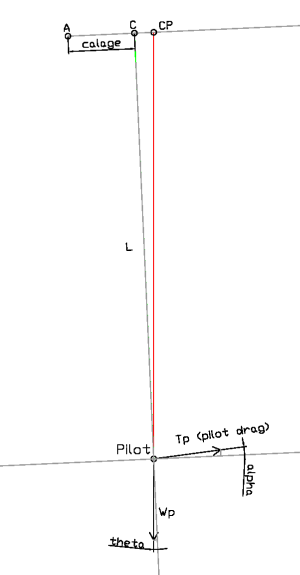
Fig. 3: Note 2
3.
Solving the system
Equilibrium equations:
[1]
q0
* Cz * δ * cos (α) +
q0
* Cxa * δ * sin (α) +
q0 * Cxs *
((L/3) * cos (α) + σ *
sin (α) ) +
q0 * Cxp
* (L * cos (α) + σ * sin (α) ) +
- mp
* g * ( L * sin (θ) + σ * cos (θ) ) +
- (l/3) * ma
* g * cos (θ) +
- q0 * Cm
= 0
[2] g * ( mp +
ma ) - q0
* ( Cz * cos (γ) + ( CxT) * sin (γ) ) = 0
[3] tan (γ) = CxT /
Cz
Auxiliar equations:
[4] q0 = (1/2) * ρ * S * V2
[5] Cxa = Cxoa +
Cxi
[6] Cxi=Cz2(α)/(π
* λ * e)
[7] λ = b2 / S
[8] CxT = Cxa + Cxs
+ Cxp
[9] Cxa = Cxoa + Cxi
[10] γ = α + θ
[11] GR = Cz / CxT
Analytical solution (to be
developed)
(...)
Numerical method:
The
solution of the system can be
obtained by analytical or by numerical method. We use the numerical
iterative way,
based on the balance equation of moments to get their sum equal to
zero. The objective is to obtain a combination of parameters to
meet the equations and provide the desired angle of glide.
Of the variables included in the
equations above consider the
following:
Inputs
ma,
mp, g, e, ρ, S, b, L, l, α
numerical estimates
Cxs, Cxp
aerodynamic values obtained
numerically
Cz, Cx, Cm, Cp
Results
V, γ, δ, θ, GR, Cxi, Cxa, CxT, q0
4. Spreadsheet
SOLVING THE EQUILIBRIUM
EQUATIONS
|
| Wing name: |
LAB_exa |
|
|
|
|
|
|
|
|
|
|
|
|
|
|
|
|
| Airfoil |
Laboratori |
|
|
|
|
|
|
|
| Surface |
25.70 |
m2 |
|
|
|
|
|
|
| Span |
10.25 |
m |
|
|
|
|
|
|
| Chord |
3.00 |
m |
|
|
|
|
|
|
| Considered chord |
3.00 |
m |
|
|
|
|
|
|
| Aspect ratio |
4.09 |
|
|
|
|
|
|
|
| Lines length |
6.00 |
m |
|
|
|
|
|
|
|
|
|
|
|
|
|
|
|
| Pilot masse |
80.00 |
Kg |
|
|
|
|
|
|
| Wing masse |
5.00 |
Kg |
|
|
|
|
|
|
|
|
|
|
|
|
|
|
|
| G |
9.81 |
m/s2 |
|
|
|
|
|
|
| RHO |
1.11 |
|
Air density |
|
|
|
|
|
| Oswald |
0.90 |
|
Oswald coeficient |
|
|
|
|
|
|
|
|
|
|
|
|
|
|
| CX pilot |
0.015 |
Pilot drag |
|
|
|
|
|
|
| CX lines |
0.020 |
Lines drag |
|
|
|
|
|
|
|
|
|
|
|
|
|
|
|
| Alfa |
5.00 |
Deg |
0.087 |
Rad |
Flight angle |
|
|
|
| Cz(alfa) |
0.900 |
Lift |
|
|
|
|
|
|
| Correcció 3D Cz |
0.624 |
|
|
|
|
|
|
|
| Cz(alfa) correction 3D |
0.562 |
|
|
|
|
|
|
|
| Cx0a(alfa) |
0.009 |
|
|
|
|
|
|
|
| Cm(alfa) |
-0.042 |
|
|
|
|
|
|
|
| Cm0 |
-0.038 |
|
|
|
|
|
|
|
| Alfa0 |
-1.700 |
|
|
|
|
|
|
|
| Cxi(alfa) |
0.070 |
|
|
cxo+ci |
Cxo |
Ci |
Cp |
Cs |
| CxT |
0.114 |
Total drag |
100.00% |
69.24% |
7.65% |
61.59% |
13.18% |
17.58% |
|
|
|
|
|
|
|
|
|
| GAMMA(alfa) |
0.200 |
Rad |
11.45 |
Deg |
4.94 |
GR |
(Cz3D) |
|
|
|
|
|
|
8.57 |
GR max |
|
|
| Theta |
0.113 |
Rad |
6.45 |
Deg |
|
|
|
|
| Q0(alfa) |
1455.1 |
|
|
|
|
|
|
|
| V |
10.09 |
m/s |
36.33 |
km/h |
Speed |
|
|
|
|
|
|
|
|
|
|
|
|
| Bl |
-0.046 |
Cm/Cz |
|
|
|
|
|
|
| Xcp |
0.296 |
Cp (%1 chord) |
|
|
|
|
|
|
| CP |
0.889 |
Cp position (m) |
|
|
|
|
|
|
| Calage |
0.433 |
Calage (m) |
|
|
|
|
|
|
| Sigma |
0.144 |
Calage chord fraction |
|
|
|
|
|
|
|
|
|
|
|
|
|
|
|
| Euilibrium of moments to
LE |
|
|
|
|
|
|
|
|
|
|
|
|
|
|
|
|
|
| M1= |
-725.02 |
|
Moment RFA |
|
|
|
|
|
| M2= |
-59.08 |
|
Moment lines |
|
|
|
|
|
| M3= |
-131.29 |
|
Moment pilot drag |
|
|
|
|
|
| M4= |
866.82 |
|
Moment pilot weight |
|
|
|
|
|
| M5= |
48.74 |
|
Moment wing weight |
|
|
|
|
|
|
|
|
|
|
|
|
|
|
| SUM= |
0.17 |
|
Zero in equilibrium |
|
|
|
|
|
|
|
|
|
|
|
|
|
|
| FH= |
0 |
|
Zero in equilibrium |
|
|
|
|
|
|
|
|
|
|
|
|
|
|
| FV= |
0 |
|
Zero in equilibrium |
|
|
|
|
|
Note: The spreadsheet is
still in development (there are some details to be
corrected). When functional the file was posted in .ods .xls
format for download.
5. Simplified equilibrium aproximation method
A
more simplified approach, although
based on the same principle of equilibrium is described below:
1. We draw the central wing profile
in the planned equilibred flight.
2. We assume that the wing is flying
with a glide ratio of GR (as
expected
for our wing), which corresponds to an angle γ
| GR |
1 |
2 |
3 |
4 |
5 |
6 |
7 |
8 |
9 |
10 |
11 |
12 |
| Angle γ (deg) |
45 |
26.57 |
18.43 |
14.04 |
11.31 |
9.46 |
8.13 |
7.13 |
6.34 |
5.71 |
5.19 |
4.76 |
3. We assume
that the airfoil incidence corresponding to max
glide ratio or slightly higher (10%), is α. Depending on the profile of
the whole wing, usually those angles ranging between 5 deg and 10 deg.
It is preferable to a plan to estimate the glide at the highest speed,
so we start by estimating the angle at 5 deg.
4. Then draw the representative
profile of the wing in flight. The
angle of the profile chord and the horizon is θ = γ - α
5. We locate the position of center
of pressure Cp for the chosen
profile and angle of incidence α.
6. We locate the position of the
pilot P in the same vertical of the
center of pressure Cp, at a distance equal to the lines length.
7. From the pilote point P draw a
perpendicular to the line of chord
wing to determine the calage
C of the wing.
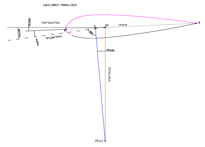
Fig. 4: The simplified
equilibrium
method
The method is simple and can be used
for a first approximation. But has
the disadvantage of having to estimate a priori the glide angle
(deductible
by the general characteristics of the wing) and the angle of attak at
maximum glide ratio (more difficult to estimate). Some corrections
on the length of the riser or lines in the prototype are necessary to
determine the calage just
ideal.
Simplified equilibrim .xls sheet.
6. Empirical methods
Many designers use empirical methods based on their experiences
with previous models. These methods are simple and effective.
A very effective method is to study the profile and the relative
length of the lines of a existing paraglider with similar
characteristics to
the project. We only need to study the middle section and deduct
graphically the
calage employee, with and
without speed system.


