PART 2: 3D-SHAPING PROGRAMMING ESTRATEGY
PART 1: Notes on the 3D formation of the leading edge in a paraglider, using ripstop fabric.
PART 2: 3D-SHAPING PROGRAMMING ESTRATEGY
PART 3: Negative 3D-shaping
PART 4: A device for experimental study of deformations and wrinkles
In this PART 2 we continue studying the concept of 3D-shaping, started in part 1.
This document shows the details and the strategy used in the
programming of the module 3D-shaping of Laboratori d'envol. We come
back to review the basics, and we propose one method in particular.
Now, we just have to move these ideas to a few lines of Fortran code,
and integrate the code within the next version of the program
LEparagliding. The work is simple. Only it is necessary to define
correctly the data, and then the logic becomes trivial. Only the part
corresponding to drawing the different parts separated, sorted and
marked, will require a detailed and hard work.
To use the program LEparagliding is not necessary to study all these
ideas... (!), these are directed only to the researchers of the details
and the concepts used inside the program. To use the program you only
need to know the meaning of some parameters that we will explain latter
in the manual.
The drawings are self explanatory (this is the intention!):

Figure 1
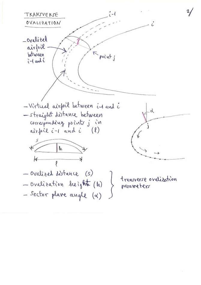
Figure 2
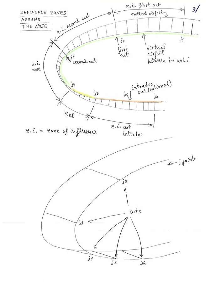
Figure 3
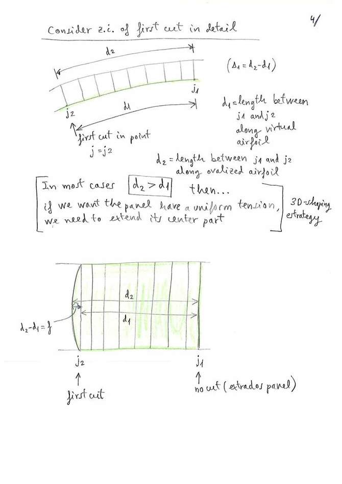
Figure 4
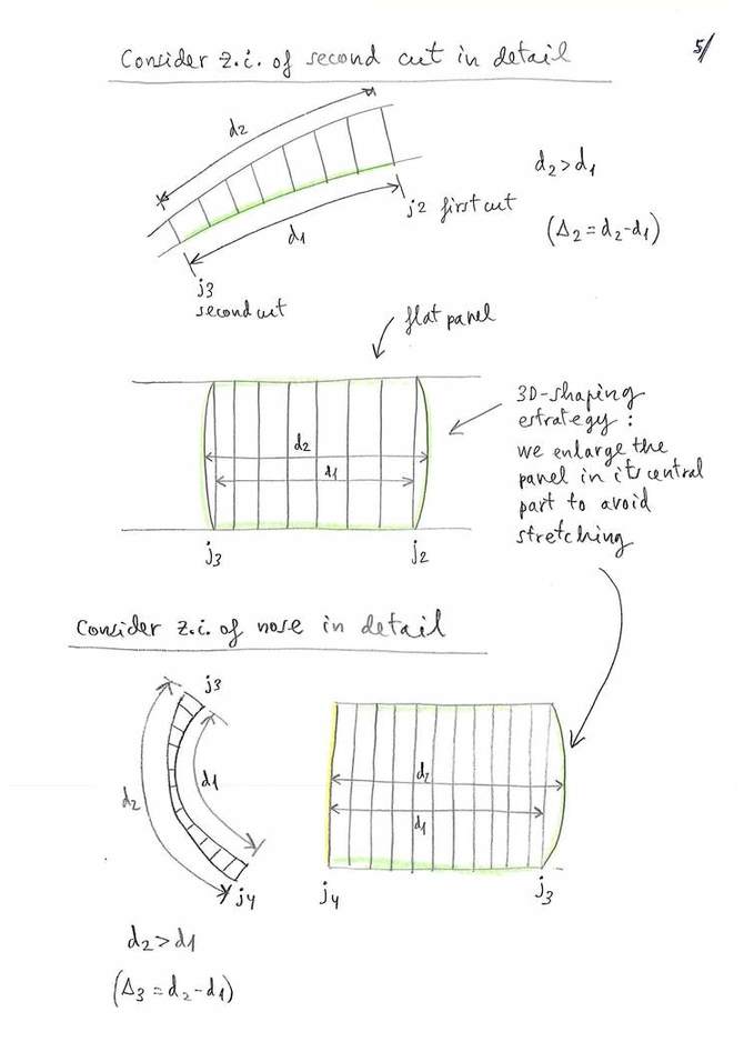
Figure 5
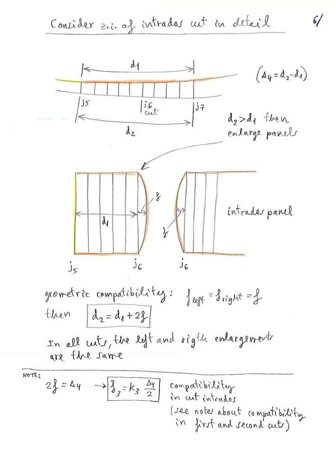
Figure 6

Figure 7
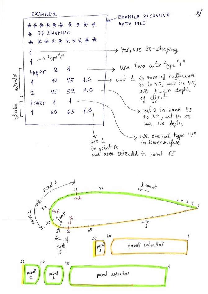
Figure 8. See note ** below
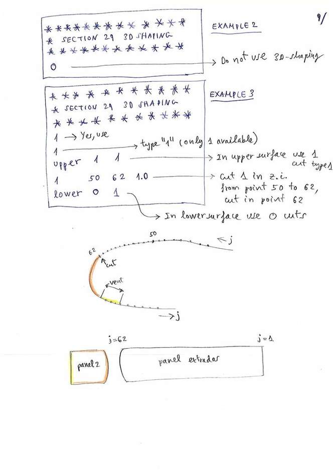
Figure 9. See note ** below
(**) Note: These examples of data are a version simplied. In the final
version we have added the concept of "groups" to define different
values for groups of profiles. Also added a few print settings of the
results to the files to dxf, and the possibility of generating other
files as well as .stl. View the last version of the LEparagliding
manual, section 29.
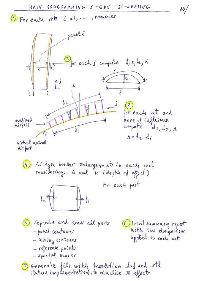
Figure 10
pdf version figures 1-10
Let's see in detail how to do calculation of the arches of the cuts (step 4 refered in figure 10):
Briefly, the system of 3D-shaping "type 1" proposed by the Laboratori
consist of making one or more transverse cuts to the panels, and add
the amount of fabric necessary to cover the "cracks" that appear on the
surfaces due to the higher thickness of the median ovalized profiles
and the pronounced curvature in the nose area.
The cracks are covered by adding arcs of fabric to the straight edges.
The arches to the right and left of the cut must be of equal length in
order to sew with a perfect match.
The arches are defined by the length of the center arrow (f).
This arrow is calculated automatically by the program, taking into
account the increases in length in the areas to the right and to the
left of the cut point. In addition, the depth of the arrow is
adjustable by the designer with a coefficient around the value 1.0. The
value 0.0 means not to apply 3D effect, the value 1.0 means to consider
the values calculated automatically, and other lower values (0.8) or
higher (1.1) reduce or amplify the 3D effect.
Consider all the points defining the profile and the following
control points in te nose area (exactly as show in figure 3 above):
j1: start reference point
j2: cut number 1 extrados
j3: cut number 2 extrados
j4: in vent
j5: out vent
j6: cut intrados
j7: end reference point
Consider the following "zones":
zone 1: between point j1 and j2
zone 2: between point j2 and j3
zone 3: between point j3 and j4
zone 4: between point j4 and j5
zone 5: between point j5 and j6
zone 6: between point j6 and j7
In each zone 1,2,3,4,5,6 (portion of panel) consider the following parameters:
d1: Length of the segment of the median airfoil without ovalization
d2: Length of the segment of the median airfoil with ovalization
d2-d1: Difference of lengths
d3: Increase of the panel at the initial edge
d4: Increase of the panel at the edge end
Now let's calculate the arrow length needed for each cut (see figures below):
- Case 0 cuts in extrados: do nothing! :)
- Case 1 cut in extrados:
We consider zone 1 beetwee point j1 and j2, and "extended zone 3" between point j2 and j4.
Let's define the arrow in cut 1 as:
f13=0.5x(d4(1)+d3(3))*k1
Where k1 is the depth coefficient around 1.0
- Case 2 cuts in extrados:
Let's define the arrow in cut 1 as:
f12=0.5x(d4(1)+d3(2))*k1
Let's define the arrow in cut 2 as:
f23=0.5x(d4(2)+d3(3))*k2
Where k1, k2 are the depth coefficients.
- Case 0 cuts in intrados: do nothing! :)
- Case 1 cut in intrados:
We consider zone 5 beetwee point j5 and j6, and zone 6 between point j6 and j7.
Let's define the arrow in cut as:
f56=0.5x(d4(5)+d3(6))*k3
Where k3 is the depth coefficient around 1.0
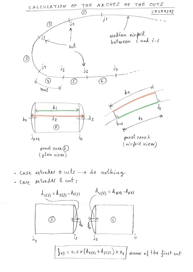
Figure 11
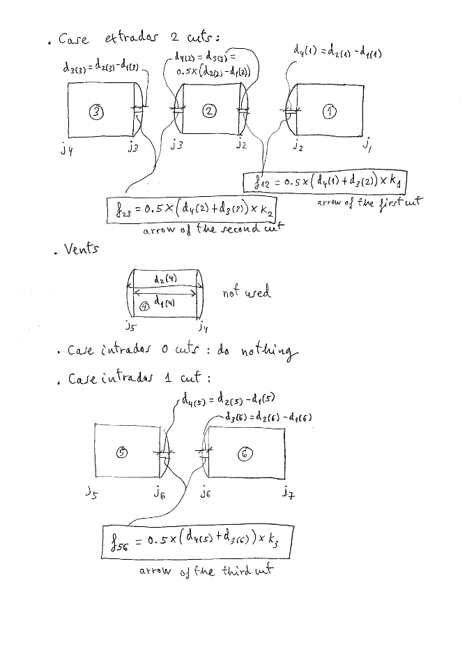
Figure 12
For each median airfoil between rib i and tip rib, program
LEparagliding computes and prints the numerical results (d1,d2,d2-d1,f)
in tabular form in the section 9 of file lep-out.txt
The next step is the drawing the arcs at the edges of the cuts...:

Figure 13. (Explanation soon...)
In relation to the step 7 programming, this is optional. But we can imagine a .DXF/.STL
tessellation file that can be visualized with OpenSCAD or FreeCAD and
will be very interesting... Crazy Idea, I imagine as possible. And yes...:
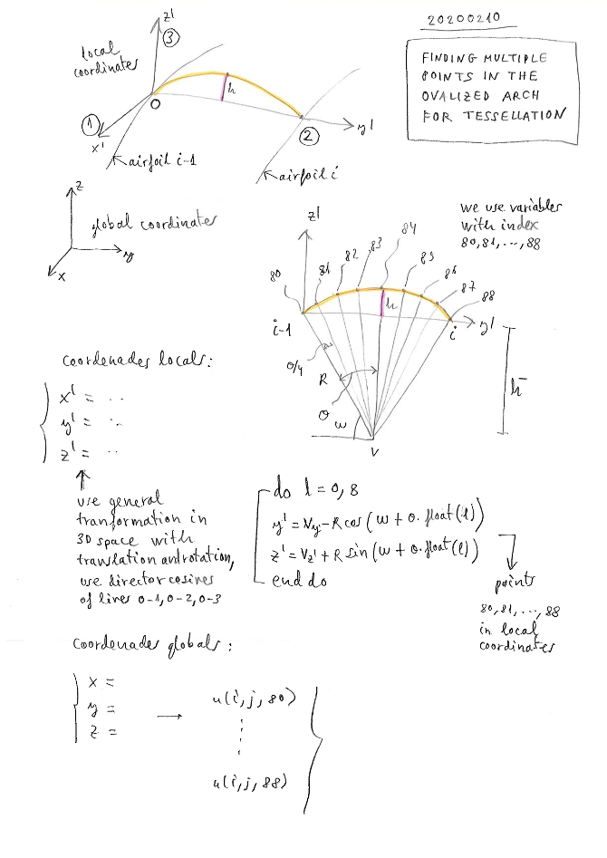
Figure 14
This page shows a simple method to define a 3D tessellation for the
ovalized surfaces. Once calculated the arc that joins the points to the
right and left of two contiguous profiles, we only need to split this
arc into smaller sections, for example 8. It is necessary to define a
local system of coordinates in the own plane of the arc, to make the
division in a simple form (for example, calculating the coordinates
relative to the center of the arc). And apply the formulas of
transformation of coordinates from local to global by translation and
rotation:

Figure 15
Now only it is necessary to convert these ideas in Fortran... :)

LEP-3.03 testing, starting code for 3D-shaping...
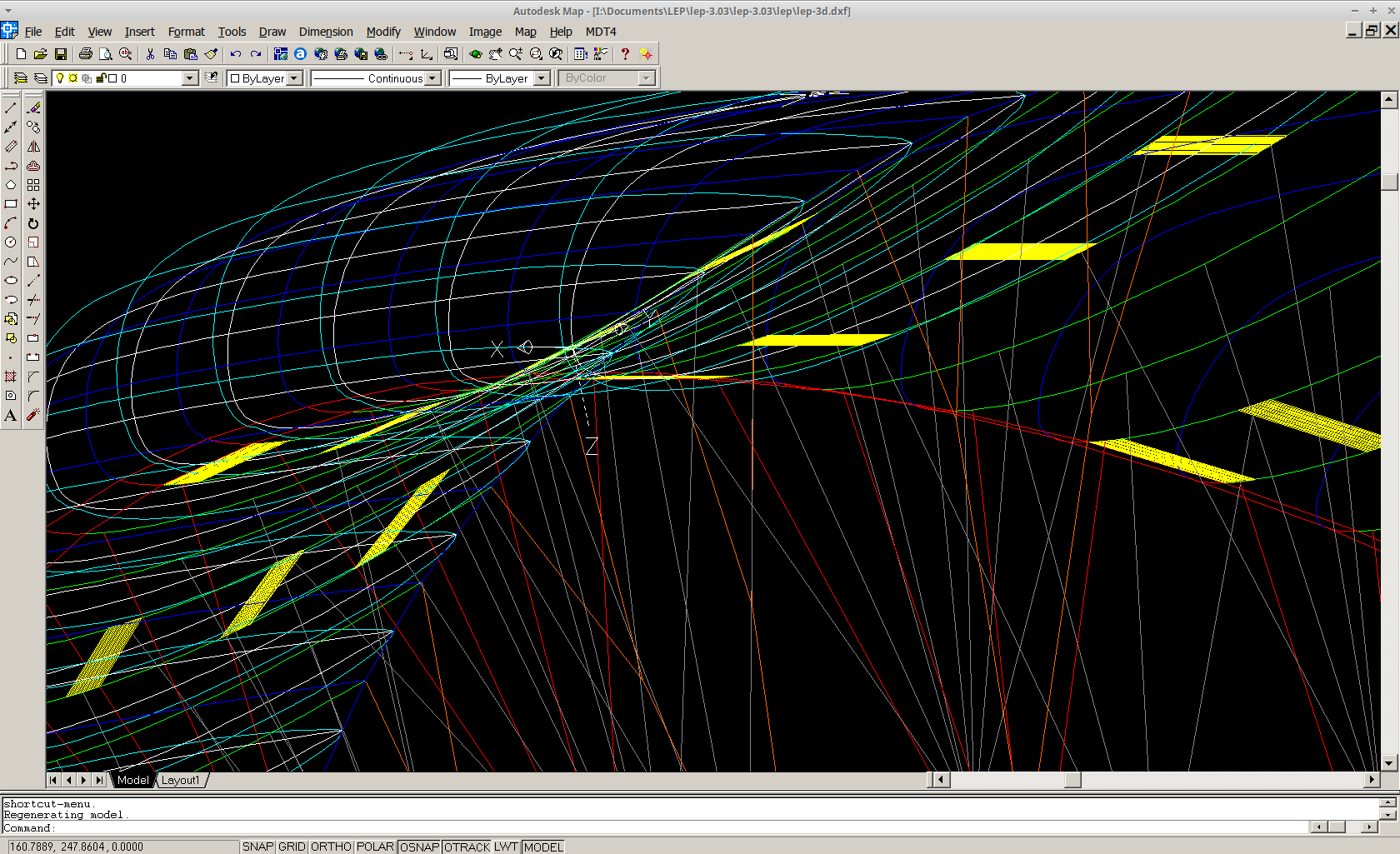
2D intermediate airfoils (white) 2D ovalized airfoils (cyan)
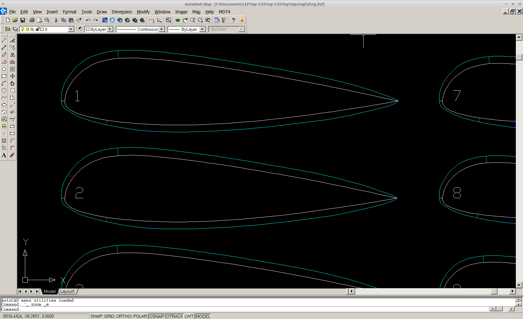
2D intermediate airfoils (white) 2D ovalized airfoils (cyan)
Module 3D-shaping for LEparagliding will be programmed in
February-March 2020 according to the plans. This plans will be possible
thanks to the support of Scott Roberts from USA (Fluid Wings https://www.fluidwings.com/ ).